Doing an On/Off analysis¶

What you will learn

You will learn how to adjust a parametrised spectral model to the events deriving the background from the data.

In classical IACT analyses the background has been normally derived from the data, by defining On (source) and Off (background) regions. An On/Off analysis is recommended if you want to assure minimal dependency on the Monte Carlo background model.

Finally, we consider the classical technique for IACT spectral analysis, in which 1D spectra for On and Off regions are used jointly to determine the source parameters.

The script csphagen is used to derive a set of On/Off observations from the event lists. This script saves the source (On) and background (Off) count spectra in OGIP format, along with the relevant information from the instrument response functions refashioned according to this format conventions.

By default, csphagen calculates the background counts using the REFLECTED algorithm, in which, for each individual observation the background regions have the same shape as the source region, and are rotated around the center of the camera keeping the same offset. As many reflected regions as possible are used, excluding the area of the camera near the source position. Since the background rates are expected to be approximately radially symmetric in camera coordinates, this method minimizes the impact of the background rate modeling from Monte Carlo. An optional exclusion map (in FITS WCS format) can be provided as input through the hidden inexclusion parameter if other regions of significant gamma-ray emission ought to be excluded from the background computation.

To derive On/Off observations from the events_edisp.fits event list, type:

$ csphagen
Input event list or observation definition XML file [obs.xml] events_edisp.fits
Calibration database [prod2]
Instrument response function [South_0.5h]
Input model definition XML file (if NONE, use point source) [NONE] $CTOOLS/share/models/crab.xml
Source name [Crab]
Algorithm for defining energy bins (FILE|LIN|LOG|POW) [LOG]
Start value for first energy bin in TeV [0.1]
Stop value for last energy bin in TeV [100.0]
Number of energy bins [120] 30
Stack multiple observations into single PHA, ARF and RMF files? [no]
Output observation definition XML file [onoff_obs.xml]
Output model definition XML file [onoff_model.xml]
Method for background estimation (REFLECTED|CUSTOM) [REFLECTED]
Coordinate system (CEL - celestial, GAL - galactic) (CEL|GAL) [CEL]
Right Ascension of source region centre (deg) (0-360) [83.63]
Declination of source region centre (deg) (-90-90) [22.01]
Radius of source region circle (deg) (0-180) [0.2]

We have provided in input a model definition file. This serves a twofold purpose: 1) a source model is used to compute the instrument response in the On region taking into account the source morphology and instrument PSF; 2) a background model is used to calculate the background response, namely the expected background rate in each energy bin and the ratio of background rate in the On region over the rate in the Off regions. You can skip using a background model by setting the hidden parameter use_model_bkg=no: in this case the background rate as a function of energy will be determined later during the fit, and the ratio of background rate in the On region over the rate in the Off regions is set to the ratio of the respective solid angles. Furthermore, you can skip passing a model definition file (pass NONE): in this case the response will be calculated for a pointlike source at the centre of the On region.

Note

We have used the events simulated accounting for energy dispersion, since energy dispersion is always used in On/Off analysis.

Note

If you wish to limit the number of observations considered to those pointed closer to the source, you can do this either at the observation selection level (see csobsselect), or directly in csphagen via the hidden maxoffset parameter.

Note

The specified parameters control the energy binning of the count spectra in reconstructed energy. For the computation of the instrument response we need a fine binning in true energy, which is controlled by the hidden parameters etruemin, etruemax, and etruebins.

The csphagen script has produced several files. The output observation definition XML file onoff_obs.xml contains a single On/Off observation:

<?xml version="1.0" encoding="UTF-8" standalone="no"?>
<observation_list title="observation list">
   <observation name="" id="" instrument="CTAOnOff" statistic="cstat">
      <parameter name="Pha_on"  file="onoff_pha_on.fits"/>
      <parameter name="Pha_off" file="onoff_pha_off.fits"/>
      <parameter name="Arf"     file="onoff_arf.fits"/>
      <parameter name="Rmf"     file="onoff_rmf.fits"/>
   </observation>
</observation_list>

Note

Note that the instrument name for an On/Off analysis is CTAOnOff. This allows combining an On/Off observations with other observation types into a single observation definition file.

The observation entails four FITS files. onoff_pha_on.fits and onoff_pha_off.fits contain the On and Off spectra, respectively. These are stored in the SPECTRUM extension of the FITS file, along with ancillary information, notably the scaling factor to be applied to the background spectrum, BACKSCAL. The third extension, EBOUNDS, contains the boundaries of the energy bins, as defined by the binning parameters in input to csphagen.

The file onoff_arf.fits contains the spectral response of the instrument extracted from the instrument response functions, including effective area for gamma-ray detection and background rates, in the SPECRESP extension. The file onoff_rmf.fits contains the remaining part of the instrument response, i.e., an energy redistribution matrix (MATRIX), as well as another instance of the EBOUNDS table. Note that we are performing a 1D analysis: the effect of the PSF is already folded into the spectral response computation.

Note

The first part of the FITS files names (and a full path to the desired location) can be set using the hidden prefix parameter of csphagen.

csphagen also produced the model definition XML file onoff_model.xml that can be directly used for model fitting:

<?xml version="1.0" encoding="UTF-8" standalone="no"?>
<source_library title="source library">
  <source name="Crab" type="PointSource">
    <spectrum type="PowerLaw">
      <parameter name="Prefactor" value="5.7" error="0" scale="1e-16" min="1e-07" max="1000" free="1" />
      <parameter name="Index" value="2.48" error="0" scale="-1" min="0" max="5" free="1" />
      <parameter name="PivotEnergy" value="0.3" scale="1000000" min="0.01" max="1000" free="0" />
    </spectrum>
    <spatialModel type="PointSource">
      <parameter name="RA" value="83.6331" scale="1" min="-360" max="360" free="0" />
      <parameter name="DEC" value="22.0145" scale="1" min="-90" max="90" free="0" />
    </spatialModel>
  </source>
  <source name="CTABackgroundModel" type="CTAIrfBackground" instrument="CTAOnOff">
    <spectrum type="PowerLaw">
      <parameter name="Prefactor" value="1" error="0" scale="1" min="0.001" max="1000" free="1" />
      <parameter name="Index" value="0" error="0" scale="1" min="-5" max="5" free="1" />
      <parameter name="PivotEnergy" value="1" scale="1000000" min="0.01" max="1000" free="0" />
    </spectrum>
  </source>
</source_library>

There are also come ancillary ds9 region files, that show the On region and the Off regions, onoff_on.reg and onoff_off.reg, respectively. Below there is a skymap where you can see the pointing direction along with the position of the On and Off regions.

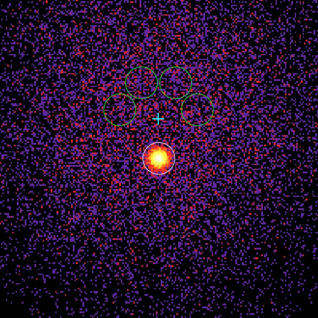
Sky map of the events. The cross shows the pointing direction, the green circles the Off regions, and the white circle the On region.

You can now fit the model onoff_model.xml using an On/Off analysis by specifying the output observation definition file and the model definition file to ctlike:

$ ctlike
Input event list, counts cube or observation definition XML file [selected_events_edisp.fits] onoff_obs.xml
Input model definition XML file [$CTOOLS/share/models/crab.xml] onoff_model.xml
Output model definition XML file [crab_results_edisp.xml] crab_results.xml

Below you see the corresponding output from the ctlike.log file. The fitted parameters are still the same within statistical uncertainties as the ones found in binned/unbinned mode. This may not always be the case, especially if the background is not well known a priori.

2019-04-02T14:55:29: +=================================+
2019-04-02T14:55:29: | Maximum likelihood optimisation |
2019-04-02T14:55:29: +=================================+
2019-04-02T14:55:29:  >Iteration   0: -logL=-47436.484, Lambda=1.0e-03
2019-04-02T14:55:29:  >Iteration   1: -logL=-47439.247, Lambda=1.0e-03, delta=2.762, step=1.0e+00, max(|grad|)=14.136296 [Index:7]
2019-04-02T14:55:29:  >Iteration   2: -logL=-47439.266, Lambda=1.0e-04, delta=0.020, step=1.0e+00, max(|grad|)=0.089563 [Index:7]
2019-04-02T14:55:29:  >Iteration   3: -logL=-47439.266, Lambda=1.0e-05, delta=0.000, step=1.0e+00, max(|grad|)=0.001727 [Index:7]
2019-04-02T14:55:29:
2019-04-02T14:55:29: +=========================================+
2019-04-02T14:55:29: | Maximum likelihood optimisation results |
2019-04-02T14:55:29: +=========================================+
2019-04-02T14:55:29: === GOptimizerLM ===
2019-04-02T14:55:29:  Optimized function value ..: -47439.266
2019-04-02T14:55:29:  Absolute precision ........: 0.005
2019-04-02T14:55:29:  Acceptable value decrease .: 2
2019-04-02T14:55:29:  Optimization status .......: converged
2019-04-02T14:55:29:  Number of parameters ......: 10
2019-04-02T14:55:29:  Number of free parameters .: 4
2019-04-02T14:55:29:  Number of iterations ......: 3
2019-04-02T14:55:29:  Lambda ....................: 1e-06
2019-04-02T14:55:29:  Maximum log likelihood ....: 47439.266
2019-04-02T14:55:29:  Observed events  (Nobs) ...: 7607.000
2019-04-02T14:55:29:  Predicted events (Npred) ..: 7606.425 (Nobs - Npred = 0.575097306655152)
2019-04-02T14:55:29: === GModels ===
2019-04-02T14:55:29:  Number of models ..........: 2
2019-04-02T14:55:29:  Number of parameters ......: 10
2019-04-02T14:55:29: === GModelSky ===
2019-04-02T14:55:29:  Name ......................: Crab
2019-04-02T14:55:29:  Instruments ...............: all
2019-04-02T14:55:29:  Observation identifiers ...: all
2019-04-02T14:55:29:  Model type ................: PointSource
2019-04-02T14:55:29:  Model components ..........: "PointSource" * "PowerLaw" * "Constant"
2019-04-02T14:55:29:  Number of parameters ......: 6
2019-04-02T14:55:29:  Number of spatial par's ...: 2
2019-04-02T14:55:29:   RA .......................: 83.6331 [-360,360] deg (fixed,scale=1)
2019-04-02T14:55:29:   DEC ......................: 22.0145 [-90,90] deg (fixed,scale=1)
2019-04-02T14:55:29:  Number of spectral par's ..: 3
2019-04-02T14:55:29:   Prefactor ................: 5.71422768206296e-16 +/- 7.28119011001326e-18 [1e-23,1e-13] ph/cm2/s/MeV (free,scale=1e-16,gradient)
2019-04-02T14:55:29:   Index ....................: -2.47772427704665 +/- 0.0108450088768338 [-0,-5]  (free,scale=-1,gradient)
2019-04-02T14:55:29:   PivotEnergy ..............: 300000 [10000,1000000000] MeV (fixed,scale=1000000,gradient)
2019-04-02T14:55:29:  Number of temporal par's ..: 1
2019-04-02T14:55:29:   Normalization ............: 1 (relative value) (fixed,scale=1,gradient)
2019-04-02T14:55:29:  Number of scale par's .....: 0
2019-04-02T14:55:29: === GCTAModelIrfBackground ===
2019-04-02T14:55:29:  Name ......................: CTABackgroundModel
2019-04-02T14:55:29:  Instruments ...............: CTAOnOff
2019-04-02T14:55:29:  Observation identifiers ...: all
2019-04-02T14:55:29:  Model type ................: "PowerLaw" * "Constant"
2019-04-02T14:55:29:  Number of parameters ......: 4
2019-04-02T14:55:29:  Number of spectral par's ..: 3
2019-04-02T14:55:29:   Prefactor ................: 0.925471278485926 +/- 0.0482291417226665 [0.001,1000] ph/cm2/s/MeV (free,scale=1,gradient)
2019-04-02T14:55:29:   Index ....................: -0.0649030558071282 +/- 0.0301870339200633 [-5,5]  (free,scale=1,gradient)
2019-04-02T14:55:29:   PivotEnergy ..............: 1000000 [10000,1000000000] MeV (fixed,scale=1000000,gradient)
2019-04-02T14:55:29:  Number of temporal par's ..: 1
2019-04-02T14:55:29:   Normalization ............: 1 (relative value) (fixed,scale=1,gradient)

ctlike has a hidden parameter called statistic that sets the statistic used for the fit. By default, ctlike will use CSTAT which is the statistic for a Poisson signal and Poisson background. When CSTAT is used, a spectral model for the signal and a spectral model for the background are jointly fit to the On and Off spectra.

Alternatively, you can use WSTAT for an On/Off analysis, which treats the number of background counts in each energy bin as a nuisance parameter that is derived from the On and Off counts by profiling the likelihood function. In this case, the only assumption is that the background rate spectrum is the same in the On and Off regions.

Note

You must use WSTAT if you have selected use_model_bkg=no in csphagen . csphagen sets automatically WSTAT as statistic in the observation definition file in this case.

Below the results for a ctlike run with the statistic=wstat option.

2019-04-02T15:56:29: +=================================+
2019-04-02T15:56:29: | Maximum likelihood optimisation |
2019-04-02T15:56:29: +=================================+
2019-04-02T15:56:29:    Parameter "Prefactor" has zero curvature. Fix parameter.
2019-04-02T15:56:29:    Parameter "Index" has zero curvature. Fix parameter.
2019-04-02T15:56:29:  >Iteration   0: -logL=13.699, Lambda=1.0e-03
2019-04-02T15:56:29:  >Iteration   1: -logL=13.645, Lambda=1.0e-03, delta=0.054, step=1.0e+00, max(|grad|)=0.226348 [Index:3]
2019-04-02T15:56:29:  >Iteration   2: -logL=13.645, Lambda=1.0e-04, delta=0.000, step=1.0e+00, max(|grad|)=0.001120 [Index:3]
2019-04-02T15:56:29:    Free parameter "Prefactor" after convergence was reached with frozen parameter.
2019-04-02T15:56:29:    Free parameter "Index" after convergence was reached with frozen parameter.
2019-04-02T15:56:29:
2019-04-02T15:56:29: +=========================================+
2019-04-02T15:56:29: | Maximum likelihood optimisation results |
2019-04-02T15:56:29: +=========================================+
2019-04-02T15:56:29: === GOptimizerLM ===
2019-04-02T15:56:29:  Optimized function value ..: 13.645
2019-04-02T15:56:29:  Absolute precision ........: 0.005
2019-04-02T15:56:29:  Acceptable value decrease .: 2
2019-04-02T15:56:29:  Optimization status .......: converged
2019-04-02T15:56:29:  Number of parameters ......: 10
2019-04-02T15:56:29:  Number of free parameters .: 4
2019-04-02T15:56:29:  Number of iterations ......: 2
2019-04-02T15:56:29:  Lambda ....................: 1e-05
2019-04-02T15:56:29:  Maximum log likelihood ....: -13.645
2019-04-02T15:56:29:  Observed events  (Nobs) ...: 7607.000
2019-04-02T15:56:29:  Predicted events (Npred) ..: 7606.133 (Nobs - Npred = 0.866926153597888)
2019-04-02T15:56:29: === GModels ===
2019-04-02T15:56:29:  Number of models ..........: 2
2019-04-02T15:56:29:  Number of parameters ......: 10
2019-04-02T15:56:29: === GModelSky ===
2019-04-02T15:56:29:  Name ......................: Crab
2019-04-02T15:56:29:  Instruments ...............: all
2019-04-02T15:56:29:  Observation identifiers ...: all
2019-04-02T15:56:29:  Model type ................: PointSource
2019-04-02T15:56:29:  Model components ..........: "PointSource" * "PowerLaw" * "Constant"
2019-04-02T15:56:29:  Number of parameters ......: 6
2019-04-02T15:56:29:  Number of spatial par's ...: 2
2019-04-02T15:56:29:   RA .......................: 83.6331 [-360,360] deg (fixed,scale=1)
2019-04-02T15:56:29:   DEC ......................: 22.0145 [-90,90] deg (fixed,scale=1)
2019-04-02T15:56:29:  Number of spectral par's ..: 3
2019-04-02T15:56:29:   Prefactor ................: 5.71398803734648e-16 +/- 7.28140878478654e-18 [1e-23,1e-13] ph/cm2/s/MeV (free,scale=1e-16,gradient)
2019-04-02T15:56:29:   Index ....................: -2.47775827196727 +/- 0.0108569325078945 [-0,-5]  (free,scale=-1,gradient)
2019-04-02T15:56:29:   PivotEnergy ..............: 300000 [10000,1000000000] MeV (fixed,scale=1000000,gradient)
2019-04-02T15:56:29:  Number of temporal par's ..: 1
2019-04-02T15:56:29:   Normalization ............: 1 (relative value) (fixed,scale=1,gradient)
2019-04-02T15:56:29:  Number of scale par's .....: 0
2019-04-02T15:56:29: === GCTAModelIrfBackground ===
2019-04-02T15:56:29:  Name ......................: CTABackgroundModel
2019-04-02T15:56:29:  Instruments ...............: CTAOnOff
2019-04-02T15:56:29:  Observation identifiers ...: all
2019-04-02T15:56:29:  Model type ................: "PowerLaw" * "Constant"
2019-04-02T15:56:29:  Number of parameters ......: 4
2019-04-02T15:56:29:  Number of spectral par's ..: 3
2019-04-02T15:56:29:   Prefactor ................: 1 +/- 0 [0.001,1000] ph/cm2/s/MeV (free,scale=1,gradient)
2019-04-02T15:56:29:   Index ....................: 0 +/- 0 [-5,5]  (free,scale=1,gradient)
2019-04-02T15:56:29:   PivotEnergy ..............: 1000000 [10000,1000000000] MeV (fixed,scale=1000000,gradient)
2019-04-02T15:56:29:  Number of temporal par's ..: 1
2019-04-02T15:56:29:   Normalization ............: 1 (relative value) (fixed,scale=1,gradient)

Warning

Beware that the profiling may yield unphysical results (negative background counts) if the number of events in the Off spectra are zero. In this case a null number of expected background events must be enforced, which can result in a bias on the source’s parameters. You can address this issue by stacking multiple observations, using a coarser energy binning, or using CSTAT instead (if you have a spectral model for the background that is good enough). See the XSPEC manual Appendix B for more information.

Note

Many scripts can also be used in On/Off mode, including ctbutterfly and csspec that were used earlier. It is sufficient to replace the input counts cube/event list with an On/Off output observation definition file to activate On/Off mode for these tools.

Previous topic

Next topic

Doing an On/Off analysis¶