Using ctools from Python
In this notebook you will learn how to use the ctools and cscripts from Python instead of typing the commands in the console.
ctools provides two Python modules that allow using all tools and
scripts as Python classes. To use ctools from Python you have to import
the ctools and cscripts modules into Python. You should also
import the gammalib module, as ctools without GammaLib is generally
not very useful.
Warning: Always import gammalib before you import ctools and
cscripts.
In [1]:
import gammalib
import ctools
import cscripts
Simulating events
As an example we will simulate an observation of an hour of the Crab nebula.
In [2]:
sim = ctools.ctobssim()
sim['inmodel']   = '${CTOOLS}/share/models/crab.xml'
sim['outevents'] = 'events.fits'
sim['caldb']     = 'prod2'
sim['irf']       = 'South_0.5h'
sim['ra']        = 83.5
sim['dec']       = 22.8
sim['rad']       = 5.0
sim['tmin']      = '2020-01-01T00:00:00'
sim['tmax']      = '2020-01-01T01:00:00'
sim['emin']      = 0.03
sim['emax']      = 150.0
sim.execute()
The first line generates an instance of the ctobssim tool as a Python
class. User parameters are then set using the [ ] operator. After
setting all parameters the execute() method is called to execute the
ctobssim tool. On output the events.fits FITS file is created.
Until now everything is analogous to running the tool from the command
line, but in Python you can easily combine the different blocks into
more complex workflows.
Remember that you can consult the manual of each tool to find out how it works and to discover all the input parameters that you can set.
In [3]:
!ctobssim --help
ctobssim
========

Simulate event list(s).


Synopsis
--------

This tool simulates event list(s) using the instrument characteristics
specified by the instrument response function(s) and an input model. The
simulation includes photon events from astrophysical sources and background
events from an instrumental background model.

By default, ctobssim creates a single event list. ctobssim queries a pointing
direction, the radius of the simulation region, a time interval, an energy
interval, an instrumental response function, and an input model. ctobssim uses
a numerical random number generator for the simulations with a seed value
provided by the hidden seed parameter. Changing this parameter for
subsequent runs will lead to different event samples.

ctobssim performs a safety check on the maximum photon rate for all model
components to avoid that the tool locks up and requests huge memory
resources, which may happen if a mistake was made in setting up the input
model (for example if an error in the flux units is made). The maximum allowed
photon rate is controlled by the hidden maxrate parameter, which by default
is set to 1e6.

ctobssim can also generate multiple event lists if an observation definition
file is specified on input using the hidden inobs parameter. In that
case, simulation information will be gathered from the file, and for each
observation an event list will be created.

For each event file, the simulation parameters will be written as data
selection keywords to the FITS header. These keywords are mandatory for any
unbinned maximum likelihood analysis of the event data.


General parameters
------------------

inobs [file]
    Input event list or observation definition XML file. If provided (i.e. the
    parameter is not blank or NONE), the pointing definition and eventually the
    response information will be extracted from the input file for event
    simulation.

inmodel [file]
    Input model XML file.

caldb [string]
    Calibration database.

irf [string]
    Instrumental response function.

(edisp = no) [boolean]
    Apply energy dispersion?

outevents [file]
    Output event list or observation definition XML file.

(prefix = sim_events_) [string]
    Prefix for event list in observation definition XML file.

(startindex = 1) [integer]
    Start index of event list in observation definition XML file.

(seed = 1) [integer]
    Integer seed value to be used for Monte Carlo simulations. Keep this
    parameter at the same value for repeatable simulations, or increment
    this value for subsequent runs if non-repeatable simulations are
    required.

ra [real]
    Right Ascension of CTA pointing (J2000, in degrees).

dec [real]
    Declination of CTA pointing (J2000, in degrees).

rad [real]
    Radius of CTA field of view (simulation cone radius) (in degrees).

tmin [time]
    Start time (UTC string, JD, MJD or MET in seconds).

tmax [time]
    Stop time (UTC string, JD, MJD or MET in seconds).

(mjdref = 51544.5) [real]
    Reference Modified Julian Day (MJD) for simulated events. The times in
    seconds for each event are counted from this reference time on.

emin [real]
    Lower energy limit of simulated events (in TeV).

emax [real]
    Upper energy limit of simulated events (in TeV).

(deadc = 0.95) [real]
    Average deadtime correction factor.

(maxrate = 1.0e6) [real]
    Maximum photon rate for source models. Source models that exceed this
    maximum photon rate will lead to an exception as very likely the
    specified model normalisation is too large (probably due to the
    a misinterpretation of units). Note that ctools specifies intensity
    units per MeV.


Standard parameters
-------------------

(nthreads = 0) [integer]
    Number of parallel processes (0=use all available CPUs).

(publish = no) [boolean]
    Specifies whether the event list(s) should be published on VO Hub.

(chatter = 2) [integer]
    Verbosity of the executable:
     chatter = 0: no information will be logged

     chatter = 1: only errors will be logged

     chatter = 2: errors and actions will be logged

     chatter = 3: report about the task execution

     chatter = 4: detailed report about the task execution

(clobber = yes) [boolean]
    Specifies whether existing files should be overwritten.

(debug = no) [boolean]
    Enables debug mode. In debug mode the executable will dump any log file output to the console.

(mode = ql) [string]
    Mode of automatic parameters (default is ql, i.e. "query and learn").

(logfile = ctobssim.log) [string]
    Name of log file.


Related tools or scripts
------------------------

csobsdef
In a Jupyter notebook a code line starting with ! is executed in the
shell, so you can do the operation above just from the command line.
One of the advantages of using ctools from Python is that you can run a tool using
In [4]:
sim.run()
The main difference to the execute() method is that the run()
method will not write the output (i.e., the simulated event list) to
disk. Why is this useful? Well, after having typed sim.run() the
ctobssim class still exists as an object in memory, including all
the simulated events. You can always save to disk later using the
save() method.
The ctobssim class has an obs() method that returns an
observation container that holds the simulated CTA observation with its
associated events. To visualise this container, type:
In [5]:
print(sim.obs())
=== GObservations ===
 Number of observations ....: 1
 Number of models ..........: 2
 Number of observed events .: 204568
 Number of predicted events : 0
There is one CTA observation in the container and to visualise that observation type:
In [6]:
print(sim.obs()[0])
=== GCTAObservation ===
 Name ......................:
 Identifier ................: 000001
 Instrument ................: CTA
 Event file ................: events.fits
 Event type ................: EventList
 Statistic .................: cstat
 Ontime ....................: 3599.99999976158 s
 Livetime ..................: 3527.99999976635 s
 Deadtime correction .......: 0.98
 User energy range .........: undefined
=== GCTAPointing ===
 Pointing direction ........: (RA,Dec)=(83.5,22.8)
=== GCTAResponseIrf ===
 Caldb mission .............: cta
 Caldb instrument ..........: prod2
 Response name .............: South_0.5h
 Energy dispersion .........: Not used
 Safe energy range .........: undefined
=== GCTAEventList ===
 Number of events ..........: 204568 (disposed in "events.fits")
 Time interval .............: 58849.0008007407 - 58849.0424674074 days
 Energy interval ...........: 0.03 - 150 TeV
 Region of interest ........: RA=83.5, DEC=22.8 [0,0] Radius=5 deg
=== GSkyRegions ===
 Number of regions .........: 0
The observation contains a CTA event list that is implement by the
GammaLib class GCTAEventList. You can access the event list using
the events() method. To visualise the individual events you can
iterate over the events using a for loop. This will show the simulated
celestial coordinates (RA, DEC), the coordinate in the camera system
[DETX, DETY], the energies and the terrestrial times (TT) of all
events. Let’s peek at the first events of the list:
In [7]:
events = sim.obs()[0].events()
for event in events[:1]:
    print(event)
Dir=RA=83.7821807861328, DEC=22.0288944244385 [-0.0134540141482956,0.00456559645656115] Energy=36.9588024914265 GeV Time=315532804.286922 s (TT)
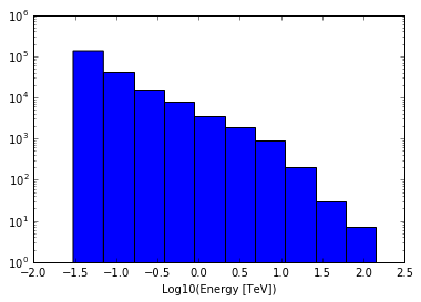
We can use this feature to inspect some of the event properties, for example look at their energy spectrum. For this we will use the Python packages matplotlib. If you do not have matplotlib you can use another plotting package of your choice or skip this step.
In [8]:
import matplotlib.pyplot as plt
%matplotlib inline
#this will visualize plots inline

ax = plt.subplot()
ax.set_yscale('log')
ax.set_xlabel('Log10(Energy [TeV])')

energies = []
for event in events:
    energies.append(event.energy().log10TeV())

n, bins, patches = plt.hist(energies)
Fitting a model to the observations
We can use the observation in memory to directly run a likelihood fit.
In [9]:
like = ctools.ctlike(sim.obs())
like.run()
This is very compact. Where do we define the model fit to the data?
Where are the user parameters? ctlike doesn’t in fact need any
parameters as all the relevant information is already contained in the
observation container produced by the ctobssim class. Indeed, you
constructed the ctlike instance by using the ctobssim observation
container as constructor argument.
An observation container, implemented by the GObservations class of
GammaLib, is the fundamental brick of any ctools analysis. An
observation container can hold more than events, e.g., in this case it
also holds the model that was used to generate the events.
Many tools and scripts handle observation containers, and accept them
upon construction and return them after running the tool via the
obs() method. Passing observation containers between ctools classes
is a very convenient and powerful way of building in-memory analysis
pipelines. However, this implies that you need some computing ressources
when dealing with large observation containers (for example if you want
to analyse a few 100 hours of data at once). Also, if the script crashes
the information is lost.
To check how the fit went you can inspect the optimiser used by
ctlike by typing:
In [10]:
print(like.opt())
=== GOptimizerLM ===
 Optimized function value ..: 766517.033
 Absolute precision ........: 0.005
 Acceptable value decrease .: 2
 Optimization status .......: converged
 Number of parameters ......: 10
 Number of free parameters .: 4
 Number of iterations ......: 2
 Lambda ....................: 1e-05
You see that the fit converged after 2 iterations. Out of 10 parameters
in the model 4 have been fitted (the others were kept fixed). To inspect
the fit results you can print the model container that can be access
using the models() method of the observation container:
In [11]:
print(like.obs().models())
=== GModels ===
 Number of models ..........: 2
 Number of parameters ......: 10
=== GModelSky ===
 Name ......................: Crab
 Instruments ...............: all
 Observation identifiers ...: all
 Model type ................: PointSource
 Model components ..........: "PointSource" * "PowerLaw" * "Constant"
 Number of parameters ......: 6
 Number of spatial par's ...: 2
  RA .......................: 83.6331 [-360,360] deg (fixed,scale=1)
  DEC ......................: 22.0145 [-90,90] deg (fixed,scale=1)
 Number of spectral par's ..: 3
  Prefactor ................: 5.71641983396841e-16 +/- 6.16044728001869e-18 [1e-23,1e-13] ph/cm2/s/MeV (free,scale=1e-16,gradient)
  Index ....................: -2.47207578184696 +/- 0.00792255637026554 [-0,-5]  (free,scale=-1,gradient)
  PivotEnergy ..............: 300000 [10000,1000000000] MeV (fixed,scale=1000000,gradient)
 Number of temporal par's ..: 1
  Normalization ............: 1 (relative value) (fixed,scale=1,gradient)
 Number of scale par's .....: 0
=== GCTAModelIrfBackground ===
 Name ......................: CTABackgroundModel
 Instruments ...............: CTA
 Observation identifiers ...: all
 Model type ................: "PowerLaw" * "Constant"
 Number of parameters ......: 4
 Number of spectral par's ..: 3
  Prefactor ................: 0.999547413672001 +/- 0.00722086618569711 [0.001,1000] ph/cm2/s/MeV (free,scale=1,gradient)
  Index ....................: -0.000149454940530402 +/- 0.00255125105744512 [-5,5]  (free,scale=1,gradient)
  PivotEnergy ..............: 1000000 [10000,1000000000] MeV (fixed,scale=1000000,gradient)
 Number of temporal par's ..: 1
  Normalization ............: 1 (relative value) (fixed,scale=1,gradient)
For example, in this way we can fetch the minimum of the optimized function (the negative of the natural logarithm of the likelihood) to compare different model hypotheses.
In [12]:
like1 = like.opt().value()
print(like1)
766517.033411
Suppose you want to repeat the fit by optimising also the position of the point source. This is easy from Python, as you can modify the model and fit interactively. Type the following:
In [13]:
like.obs().models()['Crab']['RA'].free()
like.obs().models()['Crab']['DEC'].free()
like.run()
print(like.obs().models())
=== GModels ===
 Number of models ..........: 2
 Number of parameters ......: 10
=== GModelSky ===
 Name ......................: Crab
 Instruments ...............: all
 Observation identifiers ...: all
 Model type ................: PointSource
 Model components ..........: "PointSource" * "PowerLaw" * "Constant"
 Number of parameters ......: 6
 Number of spatial par's ...: 2
  RA .......................: 83.6321513539243 +/- 0.000642709906923956 [-360,360] deg (free,scale=1)
  DEC ......................: 22.015365038759 +/- 0.000605599773766818 [-90,90] deg (free,scale=1)
 Number of spectral par's ..: 3
  Prefactor ................: 5.71414829301837e-16 +/- 6.15917760942954e-18 [1e-23,1e-13] ph/cm2/s/MeV (free,scale=1e-16,gradient)
  Index ....................: -2.47211138483201 +/- 0.0079230679574118 [-0,-5]  (free,scale=-1,gradient)
  PivotEnergy ..............: 300000 [10000,1000000000] MeV (fixed,scale=1000000,gradient)
 Number of temporal par's ..: 1
  Normalization ............: 1 (relative value) (fixed,scale=1,gradient)
 Number of scale par's .....: 0
=== GCTAModelIrfBackground ===
 Name ......................: CTABackgroundModel
 Instruments ...............: CTA
 Observation identifiers ...: all
 Model type ................: "PowerLaw" * "Constant"
 Number of parameters ......: 4
 Number of spectral par's ..: 3
  Prefactor ................: 0.999543391635431 +/- 0.0072207997895289 [0.001,1000] ph/cm2/s/MeV (free,scale=1,gradient)
  Index ....................: -0.000148647508899144 +/- 0.0025512389825989 [-5,5]  (free,scale=1,gradient)
  PivotEnergy ..............: 1000000 [10000,1000000000] MeV (fixed,scale=1000000,gradient)
 Number of temporal par's ..: 1
  Normalization ............: 1 (relative value) (fixed,scale=1,gradient)
Now we can quantify the improvement of the model by comparing the new value of the optimized function with the previous one.
In [14]:
like2 = like.opt().value()
ts    = -2.0 * (like2 - like1)
print(ts)
4.21736054635
The test statistic (TS) is expected to be distributed as a \(\chi^2_n\) with a number of degrees of freedom \(n\) equal to the additional number of degrees of freedom of the (second) more complex model with respect to the (first) more parsimonious one, for our case two degrees of freedom. The chance probability that the likelihood improved that much because of pure statistical fluctuations is the integral from TS to infinity of the chi square with two degrees of freedom. In this case the improvement is negligible (i.e., the chance probability is very high), as expected since in the model the source is already at the true position.
Generating a log file
By default, tools and scripts run from Python will not generate a log file. The reason for this is that Python scripts are often used to build ctools analysis pipelines and workflows, and one generally does not want that such a script pollutes the workspace with log files. You can however instruct a ctool or cscript to generate a log file as follows:
In [15]:
like.logFileOpen()
like.run()
This creates a log file named ctlike.log in your local work space
that you can visualise using any editor.