Performing a classical (On/Off) analysis

What you will learn

You will learn how to perform a classical analysis of a source. In this type of analysis you do not need to have a 3D (spatial and spectral) model of the irreducible background.

So far you have analysed the data in a 3-dimensional data space, spanned by position and energy, and you have used a maximum likelihood method to adjust a parametric model to the full data space. That’s the same way how Fermi-LAT data are analysed.

Traditionally, however, a different technique is used for analysing data from Imaging Air Cherenkov Telescopes. Since the irreducible background is sometimes difficult to model, it is often preferred to use the data themselves to assess the background, assuming some symmetries of the event distribution in the data space.

In ctools this method is called classical or On/Off analysis.

To execute this tutorial, create and step into a new directory:

$ mkdir my_onoff_analysis
$ cd my_onoff_analysis

Selecting the data

Let’s use the On/Off analysis method now for deriving the spectrum of a source with known position. We consider here the supernova remnant Cassiopeia A.

First, use the csobsselect script to select observations around the source of interest.

$ csobsselect
Input event list or observation definition XML file [obs.xml] $CTADATA/obs/obs_gps_baseline.xml
Pointing selection region shape (CIRCLE|BOX) [CIRCLE]
Coordinate system (CEL - celestial, GAL - galactic) (CEL|GAL) [CEL]
Right Ascension of selection centre (deg) (0-360) [83.63] 350.85
Declination of selection centre (deg) (-90-90) [22.01] 58.815
Radius of selection circle (deg) (0-180) [5.0] 2.5
Start time (UTC string, JD, MJD or MET in seconds) [NONE]
Output observation definition XML file [outobs.xml] obs.xml

Note

The offset between pointing and event directions is limited to 2.5 deg for the sake of a faster execution time for the tutorial. You can of course use a larger radius to select more observations for which the source is within the field of view, which will increase the event statistic and provide a more precise source spectrum.

Define the source and exclusion regions

Next, create a skymap to identify the source region. You do this using the ctskymap tool.

$ ctskymap
Input event list or observation definition XML file [events.fits] obs.xml
Coordinate system (CEL - celestial, GAL - galactic) (CEL|GAL) [CEL]
Projection method (AIT|AZP|CAR|GLS|MER|MOL|SFL|SIN|STG|TAN) [CAR]
First coordinate of image center in degrees (RA or galactic l) (0-360) [83.63] 350.85
Second coordinate of image center in degrees (DEC or galactic b) (-90-90) [22.01] 58.815
Image scale (in degrees/pixel) [0.02]
Size of the X axis in pixels [200] 250
Size of the Y axis in pixels [200] 250
Lower energy limit (TeV) [0.1]
Upper energy limit (TeV) [100.0] 50.0
Background subtraction method (NONE|IRF|RING) [NONE] RING
Source region radius for estimating on-counts (degrees) [0.1] 0.05
Inner background ring radius (degrees) [0.6]
Outer background ring radius (degrees) [0.8]
Number of iterations for exclusion regions computation (0-100) [0]
Output skymap file [skymap.fits]

The RING background subtraction method was used that is also a classical analysis method. For each pixel in the map the RING method estimates the background from a ring centered at the pixel. The RING method is fast and robust against linear gradients of the background rates, but requires a model (from the instrument response functions) of the background acceptance as a function of position in the field of view. You need to choose the ring inner and outer radii such that you avoid emission from a source when deriving the background. This means that the inner radius must be larger than the source’s size, or the instrument point spread function for a pointlike source.

ctskymap will produce a FITS file skymap.fits that contains three images of the region around the source. The primary image shows the excess counts, i.e., the total number of counts minus the estimated background counts. The BACKGROUND image shows the number of estimated background counts. Finally, the SIGNIFICANCE image shows the significance of the excess, calculated according to Li & Ma (1983) ApJ, 272, 317, equation 17.

You can visualize the resulting map using ds9.

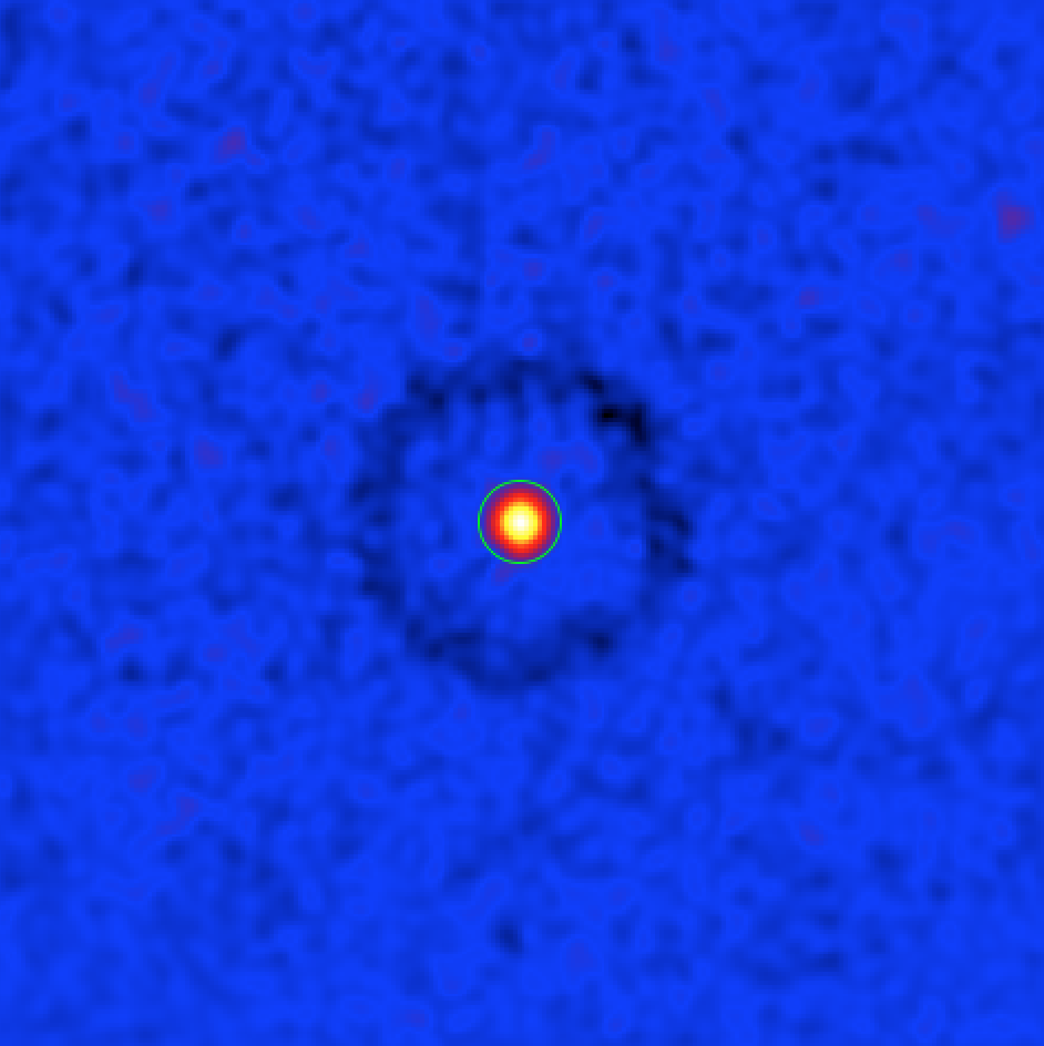
Sky map of the significance of a gamma-ray excess around Cas A. The green circle shows a circular region with 0.2 deg radius centered at the source’s position.

Note that there is a ring with negative significance (i.e., a count deficit) at offsets between 0.6 deg and 0.8 deg from the source. This is an artefact due to the fact that when computing the background for a trial source in this area the region around Cas A was falling into the ring used for the background estimation.

The artefact can be avoided by excluding the region around Cas A from the ring background estimation. To do this, let’s create an ASCII file in ds9 region format

$ nano CasA_exclusion.reg
fk5
circle(350.85,58.815,0.2)

that contains a circular region with radius 0.2 deg centered on Cas A. Alternatively, you could have created a FITS WCS map where all non-zero pixels will specify the region to be excluded.

Now re-run ctskymap with the exclusion region file provided as parameter inexclusion on the command line:

$ ctskymap inexclusion=CasA_exclusion.reg
Input event list or observation definition XML file [obs.xml]
Coordinate system (CEL - celestial, GAL - galactic) (CEL|GAL) [CEL]
Projection method (AIT|AZP|CAR|GLS|MER|MOL|SFL|SIN|STG|TAN) [CAR]
First coordinate of image center in degrees (RA or galactic l) (0-360) [350.85]
Second coordinate of image center in degrees (DEC or galactic b) (-90-90) [58.815]
Image scale (in degrees/pixel) [0.02]
Size of the X axis in pixels [250]
Size of the Y axis in pixels [250]
Lower energy limit (TeV) [0.1]
Upper energy limit (TeV) [50.0]
Background subtraction method (NONE|IRF|RING) [RING]
Source region radius for estimating on-counts (degrees) [0.05]
Inner background ring radius (degrees) [0.6]
Outer background ring radius (degrees) [0.8]
Number of iterations for exclusion regions computation (0-100) [0]
Output skymap file [skymap.fits] skymap_exclusion.fits

Below you can see the new significance map with the source exclusion region.

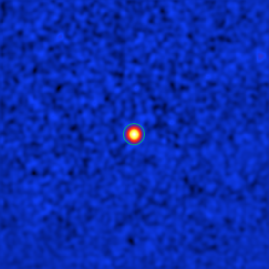
Sky map of the significance of a gamma-ray excess around Cas A. The green circle shows a circular region with 0.2 deg radius centered at the source’s position, that is excluded from the background estimation.

In fact you could have excluded Cas A from the beginning since it is a known source. In general you will need to iterate until you have found all the significant gamma-ray emission regions and added them to the exclusion regions or map, which will then be used for spectral extraction.

Note

ctskymap will automatically generate exclusion maps by collecting all sky map pixels with a significance above a given threshold in an exclusion map. Since the pixel significance will depend on the background estimate, and hence the exclusion map itself, the pixel significance needs to be iteratively recomputed after update of the exclusion map. The iterations parameter allows to specify the number of iterations (typically 3 are sufficient) and the threshold parameter specifies the significance threshold for pixels to be included in the exclusion map.

Create an On/Off observation

Now you are ready to create the source and background spectra, as well as the corresponding response files. The collection of all these files is called an On/Off observation, which has the special instrument attribute CTAOnOff in ctools. To create an On/Off observation for Cas A, run the csphagen script as follows:

$ csphagen
Input event list or observation definition XML file [obs.xml]
Input model definition XML file (if NONE, use point source) [NONE]
Algorithm for defining energy bins (FILE|LIN|LOG|POW) [LOG]
Start value for first energy bin in TeV [0.1]
Stop value for last energy bin in TeV [100.0] 50.0
Number of energy bins [120] 30
Stack multiple observations into single PHA, ARF and RMF files? [no] yes
Output observation definition XML file [onoff_obs.xml]
Output model definition XML file [onoff_model.xml]
Method for background estimation (REFLECTED|CUSTOM) [REFLECTED]
Coordinate system (CEL - celestial, GAL - galactic) (CEL|GAL) [CEL]
Right Ascension of source region centre (deg) (0-360) [83.63] 350.85
Declination of source region centre (deg) (-90-90) [22.01] 58.815
Radius of source region circle (deg) (0-180) [0.2]

The script will produce a number of output files. The central output file is the observation definition file onoff_obs.xml which looks as follows:

<?xml version="1.0" encoding="UTF-8" standalone="no"?>
<observation_list title="observation list">
  <observation name="" id="" instrument="CTAOnOff" statistic="wstat">
    <parameter name="Pha_on"  file="onoff_stacked_pha_on.fits" />
    <parameter name="Pha_off" file="onoff_stacked_pha_off.fits" />
    <parameter name="Arf"     file="onoff_stacked_arf.fits" />
    <parameter name="Rmf"     file="onoff_stacked_rmf.fits" />
  </observation>
</observation_list>

The source and background spectra are stored in so called Pulse Hight Analyzer (PHA) files with the name attributes Pha_on and Pha_off. The effective area, corrected for the angular cut, is stored in a so called Auxilliary Response File (ARF) with the name attribute Arf. The energy dispersion is stored in a so called Redistribution Matrix File (RMF) with the name attribute Rmf.

There are also some ancillary ds9 region files, that contain the On region and the Off regions for each observation, onoff_on.reg and onoff_xxx_off.reg (with xxx being the input observation identifier), respectively.

Note

In the above example you have stacked all input observations into a single On/Off observations. If you decide not to stack the observation there will be one output observation per input observation in the observation definition XML file and in the filenames the string stacked will be replaced by the observation identifier of the input observations.

Below you see a skymap showing the pointing directions along with the position of the On and Off regions for two observations (extracted from the observation definition file using the csobsinfo script).

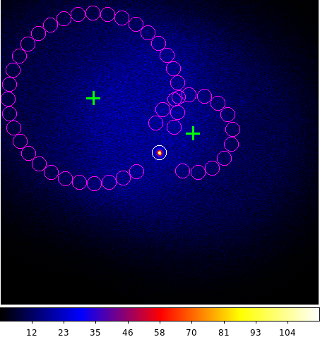
Sky map of the event counts in a larger region around Cas A (not background subtracted). The green crosses show the pointing directions, the magenta circles the Off regions, and the white circle the On region.

Fitting the On/Off observation

csphagen also generated an output model definition file onoff_model.xml than can be readily used for model fitting. Here is the content of that file:

<?xml version="1.0" encoding="UTF-8" standalone="no"?>
<source_library title="source library">
  <source name="Dummy" type="PointSource">
    <spectrum type="PowerLaw">
      <parameter name="Prefactor" value="1" error="0" scale="1e-18" min="0" free="1" />
      <parameter name="Index" value="1" error="-0" scale="-2" min="-5" max="5" free="1" />
      <parameter name="PivotEnergy" value="1" scale="1000000" free="0" />
    </spectrum>
    <spatialModel type="PointSource">
      <parameter name="RA" value="350.85" scale="1" free="0" />
      <parameter name="DEC" value="58.815" scale="1" free="0" />
    </spatialModel>
  </source>
</source_library>

Fit now the model to the data using ctlike:

$ ctlike
Input event list, counts cube or observation definition XML file [events.fits] onoff_obs.xml
Input model definition XML file [$CTOOLS/share/models/crab.xml] onoff_model.xml
Output model definition XML file [crab_results.xml] CasA_results.xml

The fit result can be inspected by peeking the log file:

2019-04-09T13:23:01: +=================================+
2019-04-09T13:23:01: | Maximum likelihood optimisation |
2019-04-09T13:23:01: +=================================+
2019-04-09T13:23:01:  >Iteration   0: -logL=808.123, Lambda=1.0e-03
2019-04-09T13:23:01:  >Iteration   1: -logL=397.528, Lambda=1.0e-03, delta=410.596, step=1.0e+00, max(|grad|)=5592.136956 [Index:3]
2019-04-09T13:23:01:  >Iteration   2: -logL=30.531, Lambda=1.0e-04, delta=366.997, step=1.0e+00, max(|grad|)=44.701876 [Index:3]
2019-04-09T13:23:01:  >Iteration   3: -logL=28.754, Lambda=1.0e-05, delta=1.777, step=1.0e+00, max(|grad|)=8.638016 [Index:3]
2019-04-09T13:23:01:  >Iteration   4: -logL=28.718, Lambda=1.0e-06, delta=0.036, step=1.0e+00, max(|grad|)=2.410274 [Index:3]
2019-04-09T13:23:01:  >Iteration   5: -logL=28.717, Lambda=1.0e-07, delta=0.001, step=1.0e+00, max(|grad|)=0.338036 [Index:3]
2019-04-09T13:23:01:
2019-04-09T13:23:01: +=========================================+
2019-04-09T13:23:01: | Maximum likelihood optimisation results |
2019-04-09T13:23:01: +=========================================+
2019-04-09T13:23:01: === GOptimizerLM ===
2019-04-09T13:23:01:  Optimized function value ..: 28.717
2019-04-09T13:23:01:  Absolute precision ........: 0.005
2019-04-09T13:23:01:  Acceptable value decrease .: 2
2019-04-09T13:23:01:  Optimization status .......: converged
2019-04-09T13:23:01:  Number of parameters ......: 6
2019-04-09T13:23:01:  Number of free parameters .: 2
2019-04-09T13:23:01:  Number of iterations ......: 5
2019-04-09T13:23:01:  Lambda ....................: 1e-08
2019-04-09T13:23:01:  Maximum log likelihood ....: -28.717
2019-04-09T13:23:01:  Observed events  (Nobs) ...: 9732.000
2019-04-09T13:23:01:  Predicted events (Npred) ..: 9685.547 (Nobs - Npred = 46.4528551491258)
2019-04-09T13:23:01: === GModels ===
2019-04-09T13:23:01:  Number of models ..........: 1
2019-04-09T13:23:01:  Number of parameters ......: 6
2019-04-09T13:23:01: === GModelSky ===
2019-04-09T13:23:01:  Name ......................: Dummy
2019-04-09T13:23:01:  Instruments ...............: all
2019-04-09T13:23:01:  Observation identifiers ...: all
2019-04-09T13:23:01:  Model type ................: PointSource
2019-04-09T13:23:01:  Model components ..........: "PointSource" * "PowerLaw" * "Constant"
2019-04-09T13:23:01:  Number of parameters ......: 6
2019-04-09T13:23:01:  Number of spatial par's ...: 2
2019-04-09T13:23:01:   RA .......................: 350.85 deg (fixed,scale=1)
2019-04-09T13:23:01:   DEC ......................: 58.815 deg (fixed,scale=1)
2019-04-09T13:23:01:  Number of spectral par's ..: 3
2019-04-09T13:23:01:   Prefactor ................: 1.40288229704921e-18 +/- 4.79754801405267e-20 [0,infty[ ph/cm2/s/MeV (free,scale=1e-18,gradient)
2019-04-09T13:23:01:   Index ....................: -2.78268915221025 +/- 0.0230642440053814 [10,-10]  (free,scale=-2,gradient)
2019-04-09T13:23:01:   PivotEnergy ..............: 1000000 MeV (fixed,scale=1000000,gradient)
2019-04-09T13:23:01:  Number of temporal par's ..: 1
2019-04-09T13:23:01:   Normalization ............: 1 (relative value) (fixed,scale=1,gradient)
2019-04-09T13:23:01:  Number of scale par's .....: 0

Tip

By default the WSTAT statistic is used which does not require a background model. If a background model should be used it needs to be provided as input model to csphagen. Here an example for an input model:

<?xml version="1.0" encoding="UTF-8" standalone="no"?>
<source_library title="source library">
  <source name="Cassiopeia A" type="PointSource">
    <spectrum type="PowerLaw">
      <parameter name="Prefactor"   value="1.45" scale="1e-18" min="0"            free="1"/>
      <parameter name="Index"       value="2.75" scale="-1"    min="-10" max="10" free="1"/>
      <parameter name="PivotEnergy" value="1"    scale="1e6"                      free="0"/>
    </spectrum>
    <spatialModel type="PointSource">
      <parameter name="RA"  value="350.8500" scale="1" free="0"/>
      <parameter name="DEC" value="58.8150"  scale="1" free="0"/>
    </spatialModel>
  </source>
  <source name="Background model" type="CTAIrfBackground" instrument="CTA">
    <spectrum type="PowerLaw">
      <parameter name="Prefactor" value="1" scale="1"   min="0.001" max="1000" free="1"/>
      <parameter name="Index"     value="0" scale="1"   min="-5"    max="5"    free="1"/>
      <parameter name="Scale"     value="1" scale="1e6" min="0.01"  max="1000" free="0"/>
    </spectrum>
  </source>
</source_library>

Now rerun csphagen as follows:

$ csphagen
Input event list or observation definition XML file [obs.xml]
Input model definition XML file (if NONE, use point source) [NONE] CasA_model.xml
Source name [Crab] Cassiopeia A
Algorithm for defining energy bins (FILE|LIN|LOG|POW) [LOG]
Start value for first energy bin in TeV [0.1]
Stop value for last energy bin in TeV [50.0]
Number of energy bins [30]
Stack multiple observations into single PHA, ARF and RMF files? [yes]
Output observation definition XML file [onoff_obs.xml] onoff_obs_cstat.xml
Output model definition XML file [onoff_model.xml] onoff_model_cstat.xml
Method for background estimation (REFLECTED|CUSTOM) [REFLECTED]
Coordinate system (CEL - celestial, GAL - galactic) (CEL|GAL) [CEL]
Right Ascension of source region centre (deg) (0-360) [350.85]
Declination of source region centre (deg) (-90-90) [58.815]
Radius of source region circle (deg) (0-180) [0.2]

This produces an observation definition file onoff_obs_cstat.xml which has the statistic attribute set to cstat:

Now you can refit the data:

$ ctlike
Input event list, counts cube or observation definition XML file [onoff_obs.xml] onoff_obs_cstat.xml
Input model definition XML file [models.xml] onoff_model_cstat.xml
Output model definition XML file [CasA_results.xml] CasA_results_cstat.xml

The fit results, which are very similar to those obtained using WSTAT before, are shown below:

2019-04-09T21:27:21: === GModelSky ===
2019-04-09T21:27:21:  Name ......................: Cassiopeia A
2019-04-09T21:27:21:  Instruments ...............: all
2019-04-09T21:27:21:  Observation identifiers ...: all
2019-04-09T21:27:21:  Model type ................: PointSource
2019-04-09T21:27:21:  Model components ..........: "PointSource" * "PowerLaw" * "Constant"
2019-04-09T21:27:21:  Number of parameters ......: 6
2019-04-09T21:27:21:  Number of spatial par's ...: 2
2019-04-09T21:27:21:   RA .......................: 350.85 deg (fixed,scale=1)
2019-04-09T21:27:21:   DEC ......................: 58.815 deg (fixed,scale=1)
2019-04-09T21:27:21:  Number of spectral par's ..: 3
2019-04-09T21:27:21:   Prefactor ................: 1.40606639795433e-18 +/- 4.84093827184383e-20 [0,infty[ ph/cm2/s/MeV (free,scale=1e-18,gradient)
2019-04-09T21:27:21:   Index ....................: -2.75705171501787 +/- 0.023581178160149 [10,-10]  (free,scale=-1,gradient)
2019-04-09T21:27:21:   PivotEnergy ..............: 1000000 MeV (fixed,scale=1000000,gradient)
2019-04-09T21:27:21:  Number of temporal par's ..: 1
2019-04-09T21:27:21:   Normalization ............: 1 (relative value) (fixed,scale=1,gradient)
2019-04-09T21:27:21:  Number of scale par's .....: 0

Visualising the source spectrum

You can visualise the source spectrum using the ctbutterfly tool and the csspec script, the first shows the uncertainty band of the fitted spectral model, while the second shows the spectral energy distribution (SED) of the source.

Like for a binned or unbinned analysis, you can create a butterfly diagram by typing

$ ctbutterfly
Input event list, counts cube or observation definition XML file [events.fits] onoff_obs.xml
Source of interest [Crab] Cassiopeia A
Input model definition XML file [$CTOOLS/share/models/crab.xml] CasA_results.xml
Lower energy limit (TeV) [0.1]
Upper energy limit (TeV) [100.0] 50.0
Output ASCII file [butterfly.txt]

and the SED by typing

$ csspec
Input event list, counts cube, or observation definition XML file [events.fits] onoff_obs.xml
Input model definition XML file [$CTOOLS/share/models/crab.xml] CasA_results.xml
Source name [Crab] Cassiopeia A
Spectrum generation method (SLICE|NODES|AUTO) [AUTO]
Binning algorithm (FILE|LIN|LOG|POW) [LOG]
Lower energy limit (TeV) [0.1]
Upper energy limit (TeV) [100.0] 50.0
Number of energy bins [20] 30
Output spectrum file [spectrum.fits]

The plot below displays the derived spectrum and butterfly

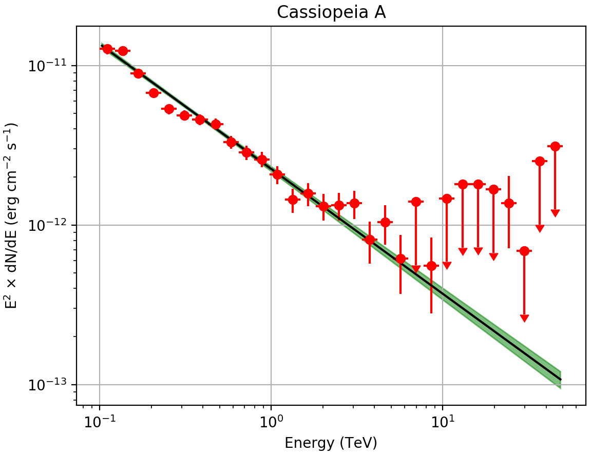
Spectral Energy Distribution of the source: the best-fit function over the whole energy range and its uncertainty range, along with the spectral points in energy bins.

To reproduce the plot download the matplotlib based script and type

$ ./show_onoff_spectrum.py