Fitting the model components to the counts cube
What you will learn
You will learn how to fit a parametric model to the counts cube using a maximum likelihood algorithm.
You will also learn how to display the fit results in form of ds9 region files, butterfly diagrams and spectral points.
Please note that display tools are not part of ctools, yet some scripts for result display that use the
matplotlibPython module can be found in the$CTOOLS/share/examples/pythonfolder (see how to display results).
Now you are ready to fit the model to the counts cube and to determine its maximum likelihood parameters.
You do this with the ctlike tool that adjusts all parameters in the
model definition file
that have the attribute free set to "1".
In the current example, the free model parameters are the positions and spectral
parameters of the two point sources and the spectral normalisation of the
background component.
You run the ctlike tool as follows:
$ ctlike
Input event list, counts cube or observation definition XML file [events.fits] cntcube.fits
Input exposure cube file [NONE] expcube.fits
Input PSF cube file [NONE] psfcube.fits
Input background cube file [NONE] bkgcube.fits
Input model definition XML file [$CTOOLS/share/models/crab.xml] bkgcube.xml
Output model definition XML file [crab_results.xml] results_stacked.xml
The tool will take a few minutes (on Mac OS X) to perform the model fitting,
and will write the results into an updated
model definition file
containing the fitted model parameters and their statistical uncertainties.
You may inspect the log file ctlike.log to verify that the model fit
converged properly, as illustrated in the example below:
2019-04-05T20:31:44: +=================================+
2019-04-05T20:31:44: | Maximum likelihood optimisation |
2019-04-05T20:31:44: +=================================+
2019-04-05T20:32:08:  >Iteration   0: -logL=293520.702, Lambda=1.0e-03
2019-04-05T20:32:32:  >Iteration   1: -logL=265518.605, Lambda=1.0e-03, delta=28002.097, step=1.0e+00, max(|grad|)=71616.018196 [Index:25]
2019-04-05T20:32:56:  >Iteration   2: -logL=259663.628, Lambda=1.0e-04, delta=5854.977, step=1.0e+00, max(|grad|)=11080.815656 [Index:3]
2019-04-05T20:33:20:  >Iteration   3: -logL=257836.468, Lambda=1.0e-05, delta=1827.160, step=1.0e+00, max(|grad|)=6857.319202 [Index:3]
2019-04-05T20:33:43:  >Iteration   4: -logL=257460.219, Lambda=1.0e-06, delta=376.249, step=1.0e+00, max(|grad|)=1834.893170 [RA:0]
2019-04-05T20:34:07:  >Iteration   5: -logL=257446.383, Lambda=1.0e-07, delta=13.836, step=1.0e+00, max(|grad|)=465.257853 [RA:0]
2019-04-05T20:34:31:  >Iteration   6: -logL=257446.252, Lambda=1.0e-08, delta=0.131, step=1.0e+00, max(|grad|)=108.665379 [RA:0]
2019-04-05T20:34:55:  >Iteration   7: -logL=257446.231, Lambda=1.0e-09, delta=0.021, step=1.0e+00, max(|grad|)=-47.972947 [RA:6]
2019-04-05T20:35:19:  >Iteration   8: -logL=257446.225, Lambda=1.0e-10, delta=0.005, step=1.0e+00, max(|grad|)=-28.053609 [RA:6]
2019-04-05T20:35:42:  >Iteration   9: -logL=257446.224, Lambda=1.0e-11, delta=0.001, step=1.0e+00, max(|grad|)=-18.165661 [RA:6]
2019-04-05T20:36:06:
2019-04-05T20:36:06: +=========================================+
2019-04-05T20:36:06: | Maximum likelihood optimisation results |
2019-04-05T20:36:06: +=========================================+
2019-04-05T20:36:06: === GOptimizerLM ===
2019-04-05T20:36:06:  Optimized function value ..: 257446.224
2019-04-05T20:36:06:  Absolute precision ........: 0.005
2019-04-05T20:36:06:  Acceptable value decrease .: 2
2019-04-05T20:36:06:  Optimization status .......: converged
2019-04-05T20:36:06:  Number of parameters ......: 28
2019-04-05T20:36:06:  Number of free parameters .: 18
2019-04-05T20:36:06:  Number of iterations ......: 9
2019-04-05T20:36:06:  Lambda ....................: 1e-12
2019-04-05T20:36:06:  Maximum log likelihood ....: -257446.224
2019-04-05T20:36:06:  Observed events  (Nobs) ...: 2069014.000
2019-04-05T20:36:06:  Predicted events (Npred) ..: 2069013.997 (Nobs - Npred = 0.00268055382184684)
You may also convert the fitted model positions into a ds9 region file using the csmodelinfo script so that you can overlay the fit results over a sky map:
$ csmodelinfo pnt_type=circle free_color=black show_labels=no
Input model definition XML file [model.xml] results_stacked.xml
Output DS9 region file [ds9.reg] positions.reg
The command line arguments pnt_type, free_color and show_labels
enable to fine tune the parameters in the ds9
region file. In this case, the positions are marked by black circles without
showing the source names.
The following image shows a zoom of the sky map that comprises both point sources, with the initial source positions determined by cssrcdetect as green crosses and the positions fitted by ctlike as black circles. Obviously, the initial positions were already near the fitted positions, which is required to assure the proper convergence of the fit.

IRF background subtracted sky map of the events recorded around the Galactic Centre during the Galactic Plane Survey with the fitted positions of the sources shown as black circles
You can also convert the spectral parameters of the point sources into a
butterfly diagram for each source using the ctbutterfly tool.
The butterfly diagram shows the envelope of all spectral models that are
statistically compatible with the data.
You create the butterfly diagram for Src001 using
$ ctbutterfly
Input event list, counts cube or observation definition XML file [events.fits] cntcube.fits
Input exposure cube file (only needed for stacked analysis) [NONE] expcube.fits
Input PSF cube file (only needed for stacked analysis) [NONE] psfcube.fits
Input background cube file (only needed for stacked analysis) [NONE] bkgcube.fits
Source of interest [Crab] Src001
Input model definition XML file [$CTOOLS/share/models/crab.xml] results_stacked.xml
Start value for first energy bin in TeV [0.1]
Stop value for last energy bin in TeV [100.0]
Output ASCII file [butterfly.txt] butterfly_src001.txt
and for Src003` using
$ ctbutterfly
Input event list, counts cube or observation definition XML file [cntcube.fits]
Input exposure cube file (only needed for stacked analysis) [expcube.fits]
Input PSF cube file (only needed for stacked analysis) [psfcube.fits]
Input background cube file (only needed for stacked analysis) [bkgcube.fits]
Source of interest [Src001] Src003
Input model definition XML file [results_stacked.xml]
Start value for first energy bin in TeV [0.1]
Stop value for last energy bin in TeV [100.0]
Output ASCII file [butterfly_src001.txt] butterfly_src003.txt
The butterfly diagrams for Src001 and Src003 are displayed in the figure
below.
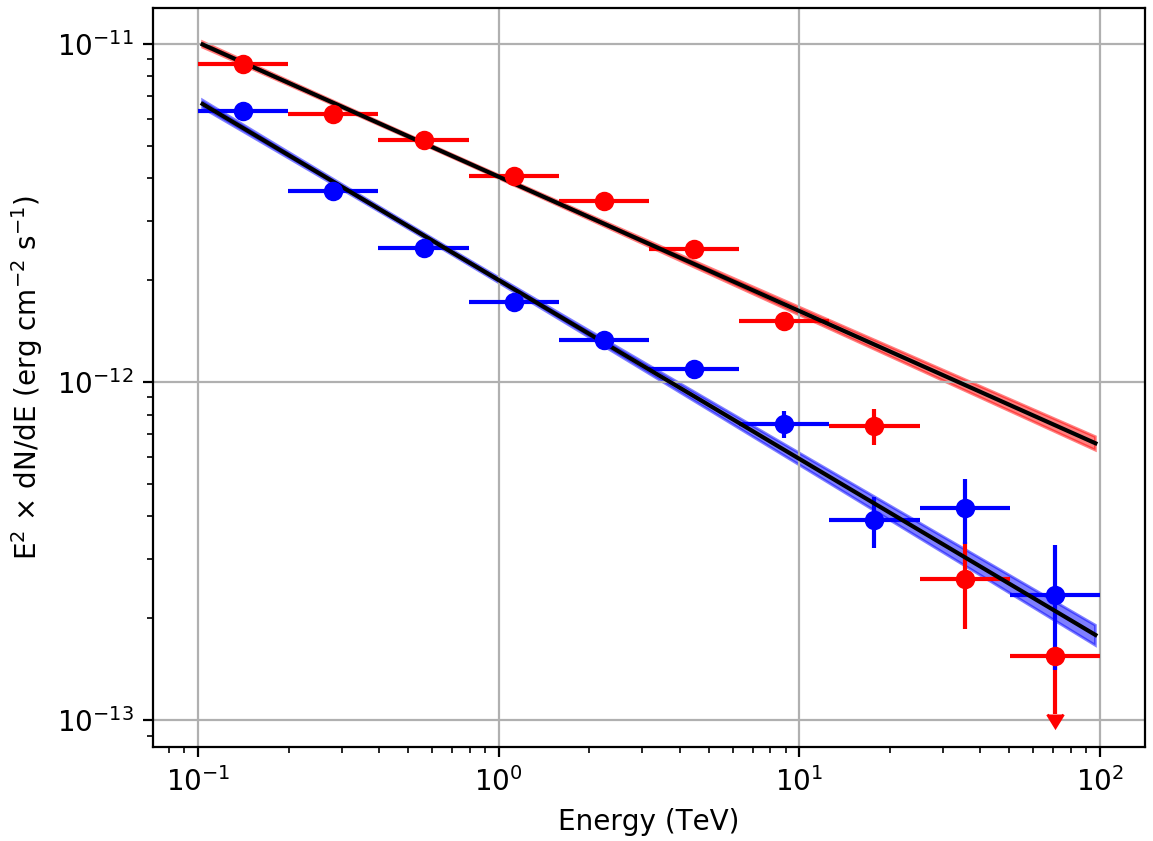
Butterfly diagrams determined with ctbutterfly and spectral points determined with csspec for Src001 (red) and Src003 (blue)
The figure also shows spectral points for each source that were determined
using the csspec script.
You create the spectrum for Src001 using
$ csspec
Input event list, counts cube, or observation definition XML file [events.fits] cntcube.fits
Input exposure cube file (only needed for stacked analysis) [NONE] expcube.fits
Input PSF cube file (only needed for stacked analysis) [NONE] psfcube.fits
Input background cube file (only needed for stacked analysis) [NONE] bkgcube.fits
Input model definition XML file [$CTOOLS/share/models/crab.xml] results_stacked.xml
Source name [Crab] Src001
Spectrum generation method (SLICE|NODES|AUTO) [AUTO]
Binning algorithm (FILE|LIN|LOG|POW) [LOG]
Lower energy limit (TeV) [0.1]
Upper energy limit (TeV) [100.0]
Number of energy bins [20] 10
Output spectrum file [spectrum.fits] spectrum_src001.fits
and for Src003 using
$ csspec
Input event list, counts cube, or observation definition XML file [cntcube.fits]
Input exposure cube file (only needed for stacked analysis) [expcube.fits]
Input PSF cube file (only needed for stacked analysis) [psfcube.fits]
Input background cube file (only needed for stacked analysis) [bkgcube.fits]
Input model definition XML file [results_stacked.xml]
Source name [Src001] Src003
Spectrum generation method (SLICE|NODES|AUTO) [AUTO]
Binning algorithm (FILE|LIN|LOG|POW) [LOG]
Lower energy limit (TeV) [0.1]
Upper energy limit (TeV) [100.0]
Number of energy bins [10]
Output spectrum file [spectrum_src001.fits] spectrum_src003.fits
The csspec script divided here the data into ten logarithmically spaced energy bins and determined the source flux in each of the bins using a maximum likelihood model fit.
Obviously, Src001 has a spectral cut-off (red flux points) and hence is not
adequately described by a power law model. You should therefore replace the
power law in the
model definition file
by an exponentially cutoff power law, as shown below:
<?xml version="1.0" encoding="UTF-8" standalone="no"?>
<source_library title="source library">
  <source name="Src001" type="PointSource">
    <spectrum type="ExponentialCutoffPowerLaw">
      <parameter name="Prefactor"    scale="1e-18" value="5.7"  min="1e-07" max="1000.0" free="1"/>
      <parameter name="Index"        scale="-1"    value="2.48" min="0.0"   max="+5.0"   free="1"/>
      <parameter name="CutoffEnergy" scale="1e7"   value="1.0"  min="0.01"  max="1000.0" free="1"/>
      <parameter name="PivotEnergy"  scale="1e6"   value="0.3"  min="0.01"  max="1000.0" free="0"/>
    </spectrum>
    <spatialModel type="PointSource">
      <parameter name="RA"  value="266.424004498437"  scale="1" free="1" />
      <parameter name="DEC" value="-29.0049010253548" scale="1" free="1" />
    </spatialModel>
  </source>
  ...
</source_library>
Fitting this model to the data improves the fit and the resulting butterfly diagram follows now reasonably well the spectral points:

Butterfly diagrams determined with ctbutterfly for an exponentially cut-off power law for Src001 (red)