The instrument response functions provide a mathematical description that links the measured quantities \(\vec{d}\) of an event to the physical quantities \(\vec{p}\) of the incident photon. The following figure illustrates this relationship:

\(I(\vec{p})\) is the gamma-ray intensity arriving at Earth as a function of photon properties \(\vec{p}\) (which usually are true photon energy, true photon incident direction, and true photon arrival time), while \(e(\vec{d})\) is the expected event rate as function of event properties \(\vec{d}\) (which usually are the measured photon energy, measured or reconstructued photon incident direction, and measured photon arrival time). The expected event rate is obtained by integrating the product of the instrumental response function \(R(\vec{d}|\vec{p},\vec{a}\)) and the emitted intensity \(I(\vec{p})\) over the photon properties \(\vec{p}\). The argument \(\vec{a}\) in the response function comprises any auxiliary parameter on which the response function may depend on (e.g. pointing direction, triggered telescopes, optical efficiencies, atmospheric conditions, etc.). All these quantities and hence the instrument response function may depend on time.
The instrument response functions for CTA are factorised into the effective area \(A_{\rm eff}(p, E, t)\) (units \(cm^2\)), the point spread function \(PSF(p' | p, E, t)\), and the energy dispersion \(E_{\rm disp}(E' | p, E, t)\) following:
ctools are shipped with response functions for the northern and southern arrays, and variants are available that have been optimised for exposure times of 0.5 hours, 5 hours and 50 hours. In total, the following six instrument response functions are available: North_0.5h, North_5h, North_50h, South_0.5h, South_5h, and South_50h.
Each response is stored in a single FITS file, and each component of the response factorisation is stored in a binary table of that FITS file. In addition, the response files contain an additional table that describes the background rate as function of energy and position in the field of view. An example of a CTA response file is shown below:
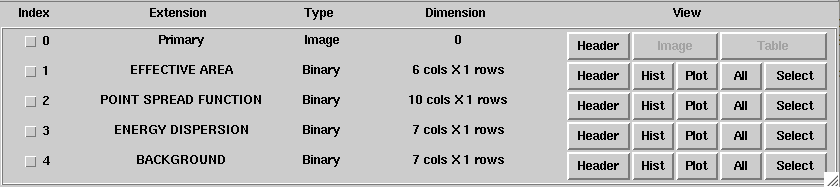
Each table in the response file is in a standardised format that is the one that is also used for the Fermi/LAT telescope. As an example, the effective area component of the response file is shown below. Response information is stored in a n-dimensional cube, and each axis of this cube is described by the lower and upper edges of the axis bins. In this example the effective area is stored as a 2D matrix with the first axis being energy and the second axis being offaxis angle. Effective area information is stored for true (EFFAREA) and reconstructed (EFFAREA_RECO) energy. Vector columns are used to store all information.

The specification of the CTA Instrument Response Functions depends on the way how ctools are used. Common to all methods is that the IRFs are defined by a response name and a calibration database name. ctools makes use of HEASARC’s CALDB format to index and store IRFs, and specification of the database and response names is sufficient to access the response.
ctools that require instrument response functions have two parameters to specify the calibration database name and the response function name. The following example shows a ctobssim run using the prod2 calibration database and the South_0.5h response function:
$ ctobssim
RA of pointing (degrees) (0-360) [83.63]
Dec of pointing (degrees) (-90-90) [22.51]
Radius of FOV (degrees) (0-180) [5.0]
Start time (MET in s) [0.0]
End time (MET in s) [1800.0]
Lower energy limit (TeV) [0.1]
Upper energy limit (TeV) [100.0]
Calibration database [prod2]
Instrument response function [South_0.5h]
Input model XML file [$CTOOLS/share/models/crab.xml]
Output event data file or observation definition XML file [events.fits]
Running the other tools is equivalent.
In the above example, only a single global response function can be used for all CTA observations. If you need to specify response functions per observation you can add the information directly in the XML observation definition file:
<observation_list title="observation library">
  <observation name="Crab" id="00001" instrument="CTA">
    <parameter name="EventList"   file="events.fits"/>
    <parameter name="Calibration" database="prod2" response="South_0.5h"/>
  </observation>
</observation_list>
The Calibration parameter specifies the calibration database and response name. You can then pass this file directly to, e.g., ctlike:
$ ctlike
Input event list, counts cube or observation definition XML file [events.fits] obs_irf.xml
Input model XML file [$CTOOLS/share/models/crab.xml]
Output model XML file [crab_results.xml]
Note that ctlike does not ask for the calibration database and response name as it found the relevant information in the XML file.
If you need even more control over individual response files, you can specify them individually in the XML observation file as follows:
<observation_list title="observation library">
  <observation name="Crab" id="00001" instrument="CTA">
    <parameter name="EventList"           file="events.fits"/>
    <parameter name="EffectiveArea"       file="$CALDB/data/cta/prod2/bcf/North_0.5h/irf_file.fits.gz"/>
    <parameter name="PointSpreadFunction" file="$CALDB/data/cta/prod2/bcf/North_0.5h/irf_file.fits.gz"/>
    <parameter name="EnergyDispersion"    file="$CALDB/data/cta/prod2/bcf/North_0.5h/irf_file.fits.gz"/>
    <parameter name="Background"          file="$CALDB/data/cta/prod2/bcf/North_0.5h/irf_file.fits.gz"/>
  </observation>
</observation_list>
The following example illustrates how to set the calibration database and response name from within Python:
import gammalib
obs   = gammalib.GCTAObservation()
caldb = gammalib.GCaldb("cta", "prod2")
irf   = "South_0.5h"
obs.response(irf, caldb)
The calibration database is set by creating a GCaldb object. The constructor takes as argument the mission (always cta) and the database name, in our case prod2. The response function is then set by passing the response name (here South_0.5h) and the calibration database object to the response method.