A central element of any data analysis is the modeling of the observed event distribution. Generally, the measured events can be separated into two distinct classes: events being attributed to gamma rays of celestial origin (the “source” events) or events being attributed to any other kind of trigger (the “background” events). In the first case, the Instrument Response Functions (IRFs) describe how an incident gamma-ray converts into a measured event. In the second case there is often no general prescription, and the distribution of background events is commonly modeled directly in the data space of the observable quantities. The main difficulty of gamma-ray astronomy is that not all events can be tagged a priori as being source or background, hence their separation can only be done on a statistical basis, based on the different morphologies, spectral characteristics or eventually temporal signatures of both event categories.
For this purpose, ctools use a general model that describes the spatial, spectral and temporal properties of the source and background components. The model is composed of an arbitrary number of model components that add up linearly to provide a prediction of the expected number of events. Model components are generally parametric, and model parameters can be adjusted through a maximum likelihood procedure to find the set of parameters that represent best the measured data. Model components representing celestial sources are convolved with the IRFs to predict the expected number of source events in the data. Background model components will be directly expressed as expected number of background events without any IRF convolution.
The general model is describe in ctools using a model definition XML file. Below is a simple example of such a file comprising one source and one background model. Each model is factorised into a spectral (tag <spectrum>), a spatial (tags <spatialModel> and <radialModel>), and a temporal component (tag <temporal>).
In this specific example, the source component Crab describes a point source at the location of the Crab nebula with a power law spectral shape that is constant in time. The background component Background is modelled as a radial Gaussian function in offset angle squared (with the offset angle being defined as the angle between pointing and measured event direction) and a spectral function that is tabulated in an ASCII file.
<?xml version="1.0" standalone="no"?>
<source_library title="source library">
  <source name="Crab" type="PointSource">
    <spatialModel type="PointSource">
      <parameter name="RA"  scale="1.0" value="83.6331" min="-360" max="360" free="1"/>
      <parameter name="DEC" scale="1.0" value="22.0145" min="-90"  max="90"  free="1"/>
    </spatialModel>
    <spectrum type="PowerLaw">
       <parameter name="Prefactor"   scale="1e-16" value="5.7"  min="1e-07" max="1000.0" free="1"/>
       <parameter name="Index"       scale="-1"    value="2.48" min="0.0"   max="+5.0"   free="1"/>
       <parameter name="PivotEnergy" scale="1e6"   value="0.3"  min="0.01"  max="1000.0" free="0"/>
    </spectrum>
    <temporal type="Constant">
      <parameter name="Normalization" scale="1.0" value="1.0" min="0.0" max="1000.0" free="0"/>
    </temporal>
  </source>
  <source name="Background" type="RadialAcceptance" instrument="CTA">
    <spectrum type="FileFunction" file="$CTOOLS/share/models/bkg_dummy.txt">
      <parameter name="Normalization" scale="1.0" value="1.0" min="0.0" max="1000.0" free="1"/>
    </spectrum>
    <radialModel type="Gaussian">
       <parameter name="Sigma" scale="1.0" value="3.0" min="0.01" max="10.0" free="1"/>
    </radialModel>
  </source>
</source_library>
Model parameters are specified by a <parameter> tag with a certain number of attributes. The name attribute gives the (case-sensitive) parameter name that needs to be unique within a given model component. The scale attribute gives a scaling factor that will be multiplied by the value attribute to provide the real (physical) parameter value. The min and max attributes specify boundaries for the value term of the parameter. And the free attribute specifies whether a parameter should be fitted (free="1") or kept fixed (free="0") in a maximum likelihood analysis. After a maximum likelihood fit using ctlike, an error attribute giving the statisical uncertainty of the value term will be appended to each <parameter> tag.
Note
For compatibility reasons with the Fermi/LAT XML format the <temporal> tag can be omitted for models that are constant in time.
Note
XML files are ASCII files and can be edited by hand using any text editor. The indentation of the XML elements is not mandatory.
Note
The splitting of parameter values into a value and scale factor is mainly for numerical purposes. Parameter fitting algorithms can be ill-conditioned if several parameters of vastly different orders of magnitudes need to be optimised simultaneously. Splitting a value into two components allows to “prescale” the parameters so that the effective parameters to be optimised (the value terms) are all of about unity.
Note
The syntax of the model definition XML file has been inspired from the syntax used by the Fermi/LAT ScienceTools, but for reasons of clarity and homogenity of the various model and parameter names we have made some modifications. Nevertheless, the format used by the Fermi/LAT ScienceTools is also supported.
The following sections present the spatial model components that are available in ctools for gamma-ray sources.
<source name="Crab" type="PointSource">
  <spatialModel type="PointSource">
    <parameter name="RA"  scale="1.0" value="83.6331" min="-360" max="360" free="1"/>
    <parameter name="DEC" scale="1.0" value="22.0145" min="-90"  max="90"  free="1"/>
  </spatialModel>
  <spectrum type="...">
    ...
  </spectrum>
</source>
Note
For compatibility with the Fermi/LAT ScienceTools the model type PointSource can be replaced by SkyDirFunction.
<source name="Crab" type="ExtendedSource">
  <spatialModel type="RadialDisk">
    <parameter name="RA"     scale="1.0" value="83.6331" min="-360" max="360" free="1"/>
    <parameter name="DEC"    scale="1.0" value="22.0145" min="-90"  max="90"  free="1"/>
    <parameter name="Radius" scale="1.0" value="0.20"    min="0.01" max="10"  free="1"/>
  </spatialModel>
  <spectrum type="...">
    ...
  </spectrum>
</source>
<source name="Crab" type="ExtendedSource"> <spatialModel type="RadialGaussian"> <parameter name="RA" scale="1.0" value="83.6331" min="-360" max="360" free="1"/> <parameter name="DEC" scale="1.0" value="22.0145" min="-90" max="90" free="1"/> <parameter name="Sigma" scale="1.0" value="0.20" min="0.01" max="10" free="1"/> </spatialModel> <spectrum type="..."> ... </spectrum> </source><source name="Crab" type="ExtendedSource"> <spatialModel type="RadialShell"> <parameter name="RA" scale="1.0" value="83.6331" min="-360" max="360" free="1"/> <parameter name="DEC" scale="1.0" value="22.0145" min="-90" max="90" free="1"/> <parameter name="Radius" scale="1.0" value="0.30" min="0.01" max="10" free="1"/> <parameter name="Width" scale="1.0" value="0.10" min="0.01" max="10" free="1"/> </spatialModel> <spectrum type="..."> ... </spectrum> </source>
<source name="Crab" type="ExtendedSource">
  <spatialModel type="EllipticalDisk">
    <parameter name="RA"          scale="1.0" value="83.6331" min="-360"  max="360" free="1"/>
    <parameter name="DEC"         scale="1.0" value="22.0145" min="-90"   max="90"  free="1"/>
    <parameter name="PA"          scale="1.0" value="45.0"    min="-360"  max="360" free="1"/>
    <parameter name="MinorRadius" scale="1.0" value="0.5"     min="0.001" max="10"  free="1"/>
    <parameter name="MajorRadius" scale="1.0" value="2.0"     min="0.001" max="10"  free="1"/>
  </spatialModel>
  <spectrum type="...">
    ...
  </spectrum>
</source>
<source name="Crab" type="ExtendedSource"> <spatialModel type="EllipticalGaussian"> <parameter name="RA" scale="1.0" value="83.6331" min="-360" max="360" free="1"/> <parameter name="DEC" scale="1.0" value="22.0145" min="-90" max="90" free="1"/> <parameter name="PA" scale="1.0" value="45.0" min="-360" max="360" free="1"/> <parameter name="MinorRadius" scale="1.0" value="0.5" min="0.001" max="10" free="1"/> <parameter name="MajorRadius" scale="1.0" value="2.0" min="0.001" max="10" free="1"/> </spatialModel> <spectrum type="..."> ... </spectrum> </source>
<source name="Crab" type="DiffuseSource">
  <spatialModel type="DiffuseIsotropic">
     <parameter name="Value" scale="1" value="1" min="1"  max="1" free="0"/>
  </spatialModel>
  <spectrum type="...">
    ...
  </spectrum>
</source>
Note
For compatibility with the Fermi/LAT ScienceTools the model type DiffuseIsotropic can be replaced by ConstantValue.
<source name="Crab" type="DiffuseSource">
  <spatialModel type="DiffuseMap" file="map.fits">
     <parameter name="Normalization" scale="1" value="1" min="0.001" max="1000.0" free="0"/>
  </spatialModel>
  <spectrum type="...">
    ...
  </spectrum>
</source>
Note
For compatibility with the Fermi/LAT ScienceTools the model type DiffuseMap can be replaced by SpatialMap and the parameter Normalization can be replaced by Prefactor.
<source name="Crab" type="DiffuseSource">
  <spatialModel type="DiffuseMapCube" file="map_cube.fits">
    <parameter name="Normalization" scale="1" value="1" min="0.001" max="1000.0" free="0"/>
  </spatialModel>
  <spectrum type="...">
    ...
  </spectrum>
</source>
Note
For compatibility with the Fermi/LAT ScienceTools the model type DiffuseMapCube can be replaced by MapCubeFunction and the parameter Normalization can be replaced by Value.
<source name="Crab" type="CompositeSource">
  <spatialModel type="Composite">
    <spatialModel type="PointSource" component="PointSource">
      <parameter name="RA"    scale="1.0" value="83.6331" min="-360" max="360" free="1"/>
      <parameter name="DEC"   scale="1.0" value="22.0145" min="-90"  max="90"  free="1"/>
    </spatialModel>
    <spatialModel type="RadialGaussian">
      <parameter name="RA"    scale="1.0" value="83.6331" min="-360" max="360" free="1"/>
      <parameter name="DEC"   scale="1.0" value="22.0145" min="-90"  max="90"  free="1"/>
      <parameter name="Sigma" scale="1.0" value="0.20"    min="0.01" max="10"  free="1"/>
    </spatialModel>
  </spatialModel>
  <spectrum type="...">
    ...
  </spectrum>
</source>
This spatial model component implements a composite model that is the sum of an arbitrary number of spatial models, computed using
\[M_{\rm spatial}(x,y|E) = \frac{1}{N} \sum_{i=0}^{N-1} M_{\rm spatial}^{(i)}(x,y|E)\]where \(M_{\rm spatial}^{(i)}(x,y|E)\) is any spatial model component (including another composite model), and \(N\) is the number of model components that are combined.
The following sections present the spatial model components that are available in ctools for background modelling.
<source name="Background" type="RadialAcceptance" instrument="CTA">
  <radialModel type="Gaussian">
    <parameter name="Sigma" scale="1.0" value="3.0" min="0.01" max="10.0" free="1"/>
  </radialModel>
  <spectrum type="...">
    ...
  </spectrum>
</source>
<source name="Background" type="RadialAcceptance" instrument="CTA"> <radialModel type="Profile"> <parameter name="Width" scale="1.0" value="1.5" min="0.1" max="1000.0" free="1"/> <parameter name="Core" scale="1.0" value="3.0" min="0.1" max="1000.0" free="1"/> <parameter name="Tail" scale="1.0" value="5.0" min="0.1" max="1000.0" free="1"/> </radialModel> <spectrum type="..."> ... </spectrum> </source><source name="Background" type="RadialAcceptance" instrument="CTA"> <radialModel type="Polynom"> <parameter name="Coeff0" scale="1.0" value="+1.00000" min="-10.0" max="10.0" free="0"/> <parameter name="Coeff1" scale="1.0" value="-0.1239176" min="-10.0" max="10.0" free="1"/> <parameter name="Coeff2" scale="1.0" value="+0.9751791" min="-10.0" max="10.0" free="1"/> <parameter name="Coeff3" scale="1.0" value="-3.0584577" min="-10.0" max="10.0" free="1"/> <parameter name="Coeff4" scale="1.0" value="+2.9089535" min="-10.0" max="10.0" free="1"/> <parameter name="Coeff5" scale="1.0" value="-1.3535372" min="-10.0" max="10.0" free="1"/> <parameter name="Coeff6" scale="1.0" value="+0.3413752" min="-10.0" max="10.0" free="1"/> <parameter name="Coeff7" scale="1.0" value="-0.0449642" min="-10.0" max="10.0" free="1"/> <parameter name="Coeff8" scale="1.0" value="+0.0024321" min="-10.0" max="10.0" free="1"/> </radialModel> <spectrum type="..."> ... </spectrum> </source>
<source name="Background" type="CTAIrfBackground" instrument="CTA">
  <spectrum type="...">
    ...
  </spectrum>
</source>
<source name="Background" type="CTACubeBackground" instrument="CTA">
  <spectrum type="...">
    ...
  </spectrum>
</source>
The following sections present the spectral model components that are available in ctools.
Warning
Source intensities are generally given in units of \({\rm ph}\,\,{\rm cm}^{-2}\,{\rm s}^{-1}\,{\rm MeV}^{-1}\).
An exception to this rule exists for the DiffuseMapCube spatial model where intensities are unitless and the spectral model presents a relative scaling of the diffuse model cube values.
If spectral models are used for a background model component, intensity units are generally given in \({\rm counts}\,\,{\rm cm}^{-2}\,{\rm s}^{-1}\,{\rm MeV}^{-1}\,{\rm sr}^{-1}\) and correspond to the on-axis count rate.
Exceptions to this rule exist for the CTAIrfBackground and CTACubeBackground models where intensities are unitless and the spectral model presents a relative scaling of the background model values.
<spectrum type="Constant">
  <parameter name="Normalization" scale="1e-16" value="5.7" min="1e-07" max="1000.0" free="1"/>
</spectrum>
This spectral model component implements the constant function
\[M_{\rm spectral}(E) = N_0\]where
- \(N_0\) = Normalization \(({\rm ph}\,\,{\rm cm}^{-2}\,{\rm s}^{-1}\,{\rm MeV}^{-1})\)
Note
For compatibility with the Fermi/LAT ScienceTools the model type Constant can be replaced by ConstantValue and the parameter Normalization by Value.
<spectrum type="PowerLaw">
  <parameter name="Prefactor"   scale="1e-16" value="5.7"  min="1e-07" max="1000.0" free="1"/>
  <parameter name="Index"       scale="-1"    value="2.48" min="0.0"   max="+5.0"   free="1"/>
  <parameter name="PivotEnergy" scale="1e6"   value="0.3"  min="0.01"  max="1000.0" free="0"/>
</spectrum>
This spectral model component implements the power law function
\[M_{\rm spectral}(E) = k_0 \left( \frac{E}{E_0} \right)^{\gamma}\]where
- \(k_0\) = Prefactor \(({\rm ph}\,\,{\rm cm}^{-2}\,{\rm s}^{-1}\,{\rm MeV}^{-1})\)
- \(\gamma\) = Index
- \(E_0\) = PivotEnergy \(({\rm MeV})\)
Warning
The PivotEnergy parameter is not intended to be fitted.
Note
For compatibility with the Fermi/LAT ScienceTools the parameter PivotEnergy can be replaced by Scale.
An alternative power law function that uses the integral photon flux as parameter rather than the Prefactor is specified by
<spectrum type="PowerLaw">
  <parameter scale="1e-07" name="PhotonFlux" min="1e-07" max="1000.0"    value="1.0" free="1"/>
  <parameter scale="1.0"   name="Index"      min="-5.0"  max="+5.0"      value="-2.0" free="1"/>
  <parameter scale="1.0"   name="LowerLimit" min="10.0"  max="1000000.0" value="100.0" free="0"/>
  <parameter scale="1.0"   name="UpperLimit" min="10.0"  max="1000000.0" value="500000.0" free="0"/>
</spectrum>
This spectral model component implements the power law function
\[M_{\rm spectral}(E) = \frac{N(\gamma+1)E^{\gamma}} {E_{\rm max}^{\gamma+1} - E_{\rm min}^{\gamma+1}}\]where
- \(N\) = PhotonFlux \(({\rm ph}\,\,{\rm cm}^{-2}\,{\rm s}^{-1})\)
- \(\gamma\) = Index
- \(E_{\rm min}\) = LowerLimit \(({\rm MeV})\)
- \(E_{\rm max}\) = UpperLimit \(({\rm MeV})\)
Warning
The LowerLimit and UpperLimit parameters are always treated as fixed and the flux given by the PhotonFlux parameter is computed over the range set by these two parameters. Use of this model allows the errors on the integral flux to be evaluated directly by ctlike.
Note
For compatibility with the Fermi/LAT ScienceTools the model type PowerLaw can be replaced by PowerLaw2 and the parameter PhotonFlux by Integral.
<spectrum type="ExponentialCutoffPowerLaw">
  <parameter name="Prefactor"    scale="1e-16" value="5.7"  min="1e-07" max="1000.0" free="1"/>
  <parameter name="Index"        scale="-1"    value="2.48" min="0.0"   max="+5.0"   free="1"/>
  <parameter name="CutoffEnergy" scale="1e6"   value="1.0"  min="0.01"  max="1000.0" free="1"/>
  <parameter name="PivotEnergy"  scale="1e6"   value="0.3"  min="0.01"  max="1000.0" free="0"/>
</spectrum>
This spectral model component implements the exponentially cut-off power law function
\[M_{\rm spectral}(E) = k_0 \left( \frac{E}{E_0} \right)^{\gamma} \exp \left( \frac{-E}{E_{\rm cut}} \right)\]where
- \(k_0\) = Prefactor \(({\rm ph}\,\,{\rm cm}^{-2}\,{\rm s}^{-1}\,{\rm MeV}^{-1})\)
- \(\gamma\) = Index
- \(E_0\) = PivotEnergy \(({\rm MeV})\)
- \(E_{\rm cut}\) = CutoffEnergy \(({\rm MeV})\)
Warning
The PivotEnergy parameter is not intended to be fitted.
Note
For compatibility with the Fermi/LAT ScienceTools the model type ExponentialCutoffPowerLaw can be replaced by ExpCutoff and the parameters CutoffEnergy by Cutoff and PivotEnergy by Scale.
<spectrum type="SuperExponentialCutoffPowerLaw">
 <parameter name="Prefactor"    scale="1e-16" value="1.0" min="1e-07" max="1000.0" free="1"/>
 <parameter name="Index1"       scale="-1"    value="2.0" min="0.0"   max="+5.0"   free="1"/>
 <parameter name="CutoffEnergy" scale="1e6"   value="1.0" min="0.01"  max="1000.0" free="1"/>
 <parameter name="Index2"       scale="1.0"   value="1.5" min="0.1"   max="5.0"    free="1"/>
 <parameter name="PivotEnergy"  scale="1e6"   value="1.0" min="0.01"  max="1000.0" free="0"/>
</spectrum>
This spectral model component implements the super exponentially cut-off power law function
\[M_{\rm spectral}(E) = k_0 \left( \frac{E}{E_0} \right)^{\gamma} \exp \left( -\left( \frac{E}{E_{\rm cut}} \right)^{\alpha} \right)\]where
- \(k_0\) = Prefactor \(({\rm ph}\,\,{\rm cm}^{-2}\,{\rm s}^{-1}\,{\rm MeV}^{-1})\)
- \(\gamma\) = Index1
- \(\alpha\) = Index2
- \(E_0\) = PivotEnergy \(({\rm MeV})\)
- \(E_{\rm cut}\) = CutoffEnergy \(({\rm MeV})\)
Warning
The PivotEnergy parameter is not intended to be fitted.
An alternative XML format is supported for compatibility with the Fermi/LAT XML format:
<spectrum type="PLSuperExpCutoff">
 <parameter name="Prefactor"   scale="1e-16" value="1.0" min="1e-07" max="1000.0" free="1"/>
 <parameter name="Index1"      scale="-1"    value="2.0" min="0.0"   max="+5.0"   free="1"/>
 <parameter name="Cutoff"      scale="1e6"   value="1.0" min="0.01"  max="1000.0" free="1"/>
 <parameter name="Index2"      scale="1.0"   value="1.5" min="0.1"   max="5.0"    free="1"/>
 <parameter name="Scale"       scale="1e6"   value="1.0" min="0.01"  max="1000.0" free="0"/>
</spectrum>
<spectrum type="BrokenPowerLaw">
  <parameter name="Prefactor"   scale="1e-16" value="5.7"  min="1e-07" max="1000.0" free="1"/>
  <parameter name="Index1"      scale="-1"    value="2.48" min="0.0"   max="+5.0"   free="1"/>
  <parameter name="BreakEnergy" scale="1e6"   value="0.3"  min="0.01"  max="1000.0" free="1"/>
  <parameter name="Index2"      scale="-1"    value="2.70" min="0.01"  max="1000.0" free="1"/>
</spectrum>
This spectral model component implements the broken power law function
\[\begin{split}M_{\rm spectral}(E) = k_0 \times \left \{ \begin{eqnarray} \left( \frac{E}{E_b} \right)^{\gamma_1} & {\rm if\,\,} E < E_b \\ \left( \frac{E}{E_b} \right)^{\gamma_2} & {\rm otherwise} \end{eqnarray} \right .\end{split}\]where
- \(k_0\) = Prefactor \(({\rm ph}\,\,{\rm cm}^{-2}\,{\rm s}^{-1}\,{\rm MeV}^{-1})\)
- \(\gamma_1\) = Index1
- \(\gamma_2\) = Index2
- \(E_b\) = BreakEnergy \(({\rm MeV})\)
Warning
Note that the BreakEnergy parameter may be poorly constrained if there is no clear spectral cut-off in the spectrum. This model may lead to complications in the maximum likelihood fitting.
Note
For compatibility with the Fermi/LAT ScienceTools the parameters BreakEnergy can be replaced by BreakValue.
<spectrum type="SmoothBrokenPowerLaw">
  <parameter name="Prefactor"       scale="1e-16" value="5.7"  min="1e-07" max="1000.0" free="1"/>
  <parameter name="Index1"          scale="-1"    value="2.48" min="0.0"   max="+5.0"   free="1"/>
  <parameter name="PivotEnergy"     scale="1e6"   value="1.0"  min="0.01"  max="1000.0" free="0"/>
  <parameter name="Index2"          scale="-1"    value="2.70" min="0.01"  max="+5.0"   free="1"/>
  <parameter name="BreakEnergy"     scale="1e6"   value="0.3"  min="0.01"  max="1000.0" free="1"/>
  <parameter name="BreakSmoothness" scale="1.0"   value="0.2"  min="0.01"  max="10.0"   free="0"/>
</spectrum>
This spectral model component implements the smoothly broken power law function
\[M_{\rm spectral}(E) = k_0 \left( \frac{E}{E_0} \right)^{\gamma_1} \left[ 1 + \left( \frac{E}{E_b} \right)^{\frac{\gamma_1 - \gamma_2}{\beta}} \right]^{-\beta}\]where
- \(k_0\) = Prefactor \(({\rm ph}\,\,{\rm cm}^{-2}\,{\rm s}^{-1}\,{\rm MeV}^{-1})\)
- \(\gamma_1\) = Index1
- \(E_0\) = PivotEnergy
- \(\gamma_2\) = Index2
- \(E_b\) = BreakEnergy \(({\rm MeV})\)
- \(\beta\) = BreakSmoothness
Warning
The pivot energy should be set far away from the expected break energy value.
Warning
When the two indices are close together, the \(\beta\) parameter becomes poorly constrained. Since the \(\beta\) parameter also scales the indices, this can cause very large errors in the estimates of the various spectral parameters. In this case, consider fixing \(\beta\).
Note
For compatibility with the Fermi/LAT ScienceTools the parameters PivotEnergy can be replaced by Scale, BreakEnergy by BreakValue and BreakSmoothness by Beta.
<spectrum type="LogParabola">
  <parameter name="Prefactor"   scale="1e-17" value="5.878"   min="1e-07" max="1000.0" free="1"/>
  <parameter name="Index"       scale="-1"    value="2.32473" min="0.0"   max="+5.0"   free="1"/>
  <parameter name="Curvature"   scale="-1"    value="0.074"   min="-5.0"  max="+5.0"   free="1"/>
  <parameter name="PivotEnergy" scale="1e6"   value="1.0"     min="0.01"  max="1000.0" free="0"/>
</spectrum>
This spectral model component implements the log parabola function
\[M_{\rm spectral}(E) = k_0 \left( \frac{E}{E_0} \right)^{\gamma+\eta \ln(E/E_0)}\]where
- \(k_0\) = Prefactor \(({\rm ph}\,\,{\rm cm}^{-2}\,{\rm s}^{-1}\,{\rm MeV}^{-1})\)
- \(\gamma\) = Index
- \(\eta\) = Curvature
- \(E_0\) = PivotEnergy \(({\rm MeV})\)
Warning
The PivotEnergy parameter is not intended to be fitted.
An alternative XML format is supported for compatibility with the Fermi/LAT XML format:
<spectrum type="LogParabola">
  <parameter name="norm"  scale="1e-17" value="5.878"   min="1e-07" max="1000.0" free="1"/>
  <parameter name="alpha" scale="1"     value="2.32473" min="0.0"   max="+5.0"   free="1"/>
  <parameter name="beta"  scale="1"     value="0.074"   min="-5.0"  max="+5.0"   free="1"/>
  <parameter name="Eb"    scale="1e6"   value="1.0"     min="0.01"  max="1000.0" free="0"/>
</spectrum>
where
- alpha = -Index
- beta = -Curvature
<spectrum type="Gaussian">
  <parameter name="Normalization" scale="1e-10" value="1.0"  min="1e-07" max="1000.0" free="1"/>
  <parameter name="Mean"          scale="1e6"   value="5.0"  min="0.01"  max="100.0"  free="1"/>
  <parameter name="Sigma"         scale="1e6"   value="1.0"  min="0.01"  max="100.0"  free="1"/>
</spectrum>
This spectral model component implements the gaussian function
\[M_{\rm spectral}(E) = \frac{N_0}{\sqrt{2\pi}\sigma} \exp \left( \frac{-(E-\bar{E})^2}{2 \sigma^2} \right)\]where
- \(N_0\) = Normalization \(({\rm ph}\,\,{\rm cm}^{-2}\,{\rm s}^{-1})\)
- \(\bar{E}\) = Mean \(({\rm MeV})\)
- \(\sigma\) = Sigma \(({\rm MeV})\)
<spectrum type="FileFunction" file="data/filefunction.txt">
  <parameter scale="1.0" name="Normalization" min="0.0" max="1000.0" value="1.0" free="1"/>
</spectrum>
This spectral model component implements an arbitrary function that is defined by intensity values at specific energies. The energy and intensity values are defined using an ASCII file with columns of energy and differential flux values. Energies are given in units of \({\rm MeV}\), intensities are given in units of \({\rm ph}\,\,{\rm cm}^{-2}\,{\rm s}^{-1}\,{\rm MeV}^{-1}\). The only parameter is a multiplicative normalization:
\[M_{\rm spectral}(E) = N_0 \left. \frac{dN}{dE} \right\rvert_{\rm file}\]where
- \(N_0\) = Normalization
Warning
If the file name is given without a path it is expected that the file resides in the same directory than the XML file. If the file resides in a different directory, an absolute path name should be specified. Any environment variable present in the path name will be expanded.
<spectrum type="NodeFunction">
  <node>
    <parameter name="Energy"    scale="1.0"   value="1.0" min="0.1"   max="1.0e20" free="0"/>
    <parameter name="Intensity" scale="1e-07" value="1.0" min="1e-07" max="1000.0" free="1"/>
  </node>
  <node>
    <parameter name="Energy"    scale="10.0"  value="1.0" min="0.1"   max="1.0e20" free="0"/>
    <parameter name="Intensity" scale="1e-08" value="1.0" min="1e-07" max="1000.0" free="1"/>
  </node>
</spectrum>
This spectral model component implements a generalised broken power law which is defined by a set of energy and intensity values (the so called nodes) that are piecewise connected by power laws. Energies are given in units of \({\rm MeV}\), intensities are given in units of \({\rm ph}\,\,{\rm cm}^{-2}\,{\rm s}^{-1}\,{\rm MeV}^{-1}\).
Warning
An arbitrary number of energy-intensity nodes can be defined in a node function. The nodes need to be sorted by increasing energy. Although the fitting of the Energy parameters is formally possible it may lead to numerical complications. If Energy parameters are to be fitted make sure that the min and max attributes are set in a way that avoids inversion of the energy ordering.
<spectrum type="Composite">
  <spectrum type="PowerLaw" component="SoftComponent">
    <parameter name="Prefactor"   scale="1e-17" value="3"  min="1e-07" max="1000.0" free="1"/>
    <parameter name="Index"       scale="-1"    value="3.5" min="0.0"   max="+5.0"   free="1"/>
    <parameter name="PivotEnergy" scale="1e6"   value="1"  min="0.01"  max="1000.0" free="0"/>
  </spectrum>
  <spectrum type="PowerLaw" component="HardComponent">
    <parameter name="Prefactor"   scale="1e-17" value="5"  min="1e-07" max="1000.0" free="1"/>
    <parameter name="Index"       scale="-1"    value="2.0" min="0.0"   max="+5.0"   free="1"/>
    <parameter name="PivotEnergy" scale="1e6"   value="1"  min="0.01"  max="1000.0" free="0"/>
  </spectrum>
</spectrum>
This spectral model component implements a composite model that is the sum of an arbitrary number of spectral models, computed using
\[M_{\rm spectral}(E) = \sum_{i=0}^{N-1} M_{\rm spectral}^{(i)}(E)\]where \(M_{\rm spectral}^{(i)}(E)\) is any spectral model component (including another composite model), and \(N\) is the number of model components that are combined.
<spectrum type="Multiplicative">
  <spectrum type="PowerLaw" component="PowerLawComponent">
    <parameter name="Prefactor"   scale="1e-17" value="1.0"  min="1e-07" max="1000.0" free="1"/>
    <parameter name="Index"       scale="-1"    value="2.48" min="0.0"   max="+5.0"   free="1"/>
    <parameter name="PivotEnergy" scale="1e6"   value="1.0"  min="0.01"  max="1000.0" free="0"/>
  </spectrum>
  <spectrum type="ExponentialCutoffPowerLaw" component="CutoffComponent">
    <parameter name="Prefactor"    scale="1.0" value="1.0" min="1e-07" max="1000.0" free="0"/>
    <parameter name="Index"        scale="1.0" value="0.0" min="-2.0"  max="+2.0"   free="0"/>
    <parameter name="CutoffEnergy" scale="1e6" value="1.0" min="0.01"  max="1000.0" free="1"/>
    <parameter name="PivotEnergy"  scale="1e6" value="1.0" min="0.01"  max="1000.0" free="0"/>
  </spectrum>
</spectrum>
This spectral model component implements a composite model that is the product of an arbitrary number of spectral models, computed using
\[M_{\rm spectral}(E) = \prod_{i=0}^{N-1} M_{\rm spectral}^{(i)}(E)\]where \(M_{\rm spectral}^{(i)}(E)\) is any spectral model component (including another composite model), and \(N\) is the number of model components that are multiplied.
The following sections present the temporal model components that are available in ctools.
<temporal type="Constant">
  <parameter name="Normalization" scale="1.0" value="1.0" min="0.1" max="10.0" free="0"/>
</temporal>
This temporal model component implements a constant source
\[M_{\rm temporal}(t) = N_0\]where
- \(N_0\) = Normalization
<temporal type="LightCurve" file="model_temporal_lightcurve.fits">
  <parameter name="Normalization" scale="1" value="1.0" min="0.0" max="1000.0" free="0"/>
</temporal>
This temporal model component implements a light curve \(r(t)\)
\[M_{\rm temporal}(t) = N_0 \times r(t)\]where
- \(N_0\) = Normalization
The light curve is defined by nodes in a FITS file that specify the relative flux normalization as function of time (file model_temporal_lightcurve.fits in the example above). The structure of the light curve FITS file is shown in the figure below. The light curve is defined in the first extension of the FITS file and consists of a binary table with the columns TIME and NORM. Times in the TIME columns are given in seconds and are counted with respect to a time reference that is defined in the header of the binary table. Times need to be specified in ascending order. The values in the NORM column specify \(r(t)\) at times \(t\), and should be comprised between 0 and 1.
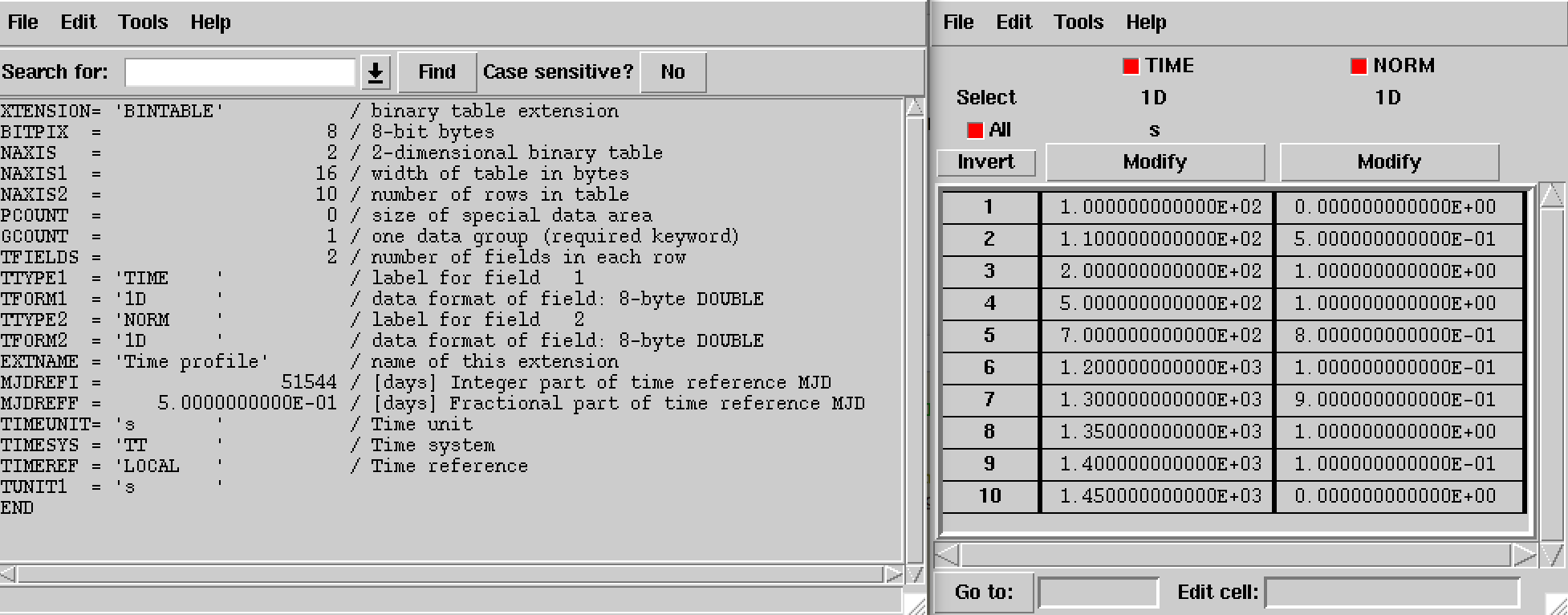
Structure of light curve FITS file
Warning
Fitting of light curves only makes sense for an unbinned maximum likelihood analysis, since in a binned or stacked analysis the times of individual events are dropped.
<temporal type="PhaseCurve" file="model_temporal_phasecurve.fits">
  <parameter name="Normalization" scale="1" value="1.0"     min="0.0" max="1000.0"   free="0"/>
  <parameter name="MJD"           scale="1" value="51544.5" min="0.0" max="100000.0" free="0"/>
  <parameter name="Phase"         scale="1" value="0.0"     min="0.0" max="1.0"      free="0"/>
  <parameter name="F0"            scale="1" value="1.0"     min="0.0" max="1000.0"   free="0"/>
  <parameter name="F1"            scale="1" value="0.1"     min="0.0" max="1000.0"   free="0"/>
  <parameter name="F2"            scale="1" value="0.01"    min="0.0" max="1000.0"   free="0"/>
</temporal>
This temporal model component implements a phase curve \(r(\Phi(t))\)
\[M_{\rm temporal}(t) = N_0 \times r(\Phi(t))\]where the phase as function of time is computed using
\[\Phi(t) = \Phi_0 + f(t-t_0) + \frac{1}{2}\dot{f} (t-t_0)^2 + \frac{1}{6}\ddot{f} (t-t_0)^3\]and
- \(N_0\) = Normalization
- \(t_0\) = MJD
- \(\Phi_0\) = Phase
- \(f\) = F0
- \(\dot{f}\) = F1
- \(\ddot{f}\) = F2
The phase curve is defined by nodes in a FITS file that specify the relative flux normalization as function of phase (file model_temporal_phasecurve.fits in the example above). The structure of the phase curve FITS file is shown in the figure below. The phase curve is defined in the first extension of the FITS file and consists of a binary table with the columns PHASE and NORM. Phase values in the PHASE column need to be comprised between 0 and 1 and need to be given in ascending order. The values in the NORM column specify \(r(\Phi(t))\) at phases \(\Phi(t)\), and should be comprised between 0 and 1.
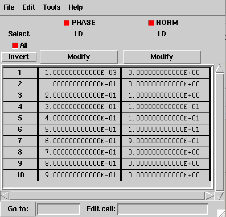
Structure of phase curve FITS file
Warning
Fitting of phase curves only makes sense for an unbinned maximum likelihood analysis, since in a binned or stacked analysis the times of individual events are dropped.
Warning
Fitting of phase curve parameters may not properly work for pulsar frequencies.