How to jointly analyse data from different instruments?

What you will learn

You will learn how to jointly analyse data from different instruments.

In this tutorial you will learn how to jointly analyse data observed with Fermi-LAT and simulated data for CTA for the Vela pulsar and pulsar wind nebula.

Prepare Fermi-LAT data

The preparation of Fermi-LAT data will follow the description provided on Prepare Fermi-LAT data.

Prepare CTA data

For CTA the simulations of the Galactic Plane Scan from the first Data Challenge will be used. First, select all observations from the data with pointing directions close to the Vela pulsar:

$ csobsselect
Input event list or observation definition XML file [obs.xml] $CTADATA/obs/obs_gps_baseline.xml
Pointing selection region shape (CIRCLE|BOX) [CIRCLE]
Coordinate system (CEL - celestial, GAL - galactic) (CEL|GAL) [CEL]
Right Ascension of selection centre (deg) (0-360) [83.63] 128.838
Declination of selection centre (deg) (-90-90) [22.01] -45.178
Radius of selection circle (deg) (0-180) [5.0]
Start time (UTC string, JD, MJD or MET in seconds) [NONE]
Output observation definition XML file [outobs.xml] obs_vela.xml

Then bin the selected observations into a counts cube

$ ctbin
Input event list or observation definition XML file [events.fits] obs_vela.xml
Coordinate system (CEL - celestial, GAL - galactic) (CEL|GAL) [CEL]
Projection method (AIT|AZP|CAR|GLS|MER|MOL|SFL|SIN|STG|TAN) [CAR]
First coordinate of image center in degrees (RA or galactic l) (0-360) [83.63] 128.838
Second coordinate of image center in degrees (DEC or galactic b) (-90-90) [22.51] -45.178
Image scale (in degrees/pixel) [0.02]
Size of the X axis in pixels [200]
Size of the Y axis in pixels [200]
Algorithm for defining energy bins (FILE|LIN|LOG|POW) [LOG]
Lower energy limit (TeV) [0.1] 0.03
Upper energy limit (TeV) [100.0] 150.0
Number of energy bins (1-200) [20] 40
Output counts cube file [cntcube.fits]

Then compute the response cubes as follows

$ ctexpcube
Input event list or observation definition XML file [NONE] obs_vela.xml
Input counts cube file to extract exposure cube definition [NONE] cntcube.fits
Output exposure cube file [expcube.fits]

$ ctpsfcube
Input event list or observation definition XML file [NONE] obs_vela.xml
Input counts cube file to extract PSF cube definition [NONE]
Coordinate system (CEL - celestial, GAL - galactic) (CEL|GAL) [CEL]
Projection method (AIT|AZP|CAR|GLS|MER|MOL|SFL|SIN|STG|TAN) [CAR]
First coordinate of image center in degrees (RA or galactic l) (0-360) [83.63] 128.838
Second coordinate of image center in degrees (DEC or galactic b) (-90-90) [22.51] -45.178
Image scale (in degrees/pixel) [1.0]
Size of the X axis in pixels [10]
Size of the Y axis in pixels [10]
Algorithm for defining energy bins (FILE|LIN|LOG|POW) [LOG]
Lower energy limit (TeV) [0.1] 0.03
Upper energy limit (TeV) [100.0] 150.0
Number of energy bins (1-200) [20] 40
Output PSF cube file [psfcube.fits]

$ ctbkgcube
Input event list or observation definition XML file [NONE] obs_vela.xml
Input counts cube file to extract background cube definition [NONE] cntcube.fits
Input model definition XML file [NONE] $CTOOLS/share/models/bkg_irf.xml
Output background cube file [bkgcube.fits]
Output model definition XML file [NONE] bkgcube.xml

Combining the observations

Now you have all the data and hand. You have to create an observation definition file to combine the data for an analysis:

<?xml version="1.0" standalone="no"?>
<observation_list title="observation library">
  <observation name="Vela" id="000001" instrument="CTA">
    <parameter name="CountsCube"   file="cntcube.fits"/>
    <parameter name="ExposureCube" file="expcube.fits"/>
    <parameter name="PsfCube"      file="psfcube.fits"/>
    <parameter name="BkgCube"      file="bkgcube.fits"/>
  </observation>
  <observation name="Vela" id="000001" instrument="LAT">
    <parameter name="CountsMap"    file="srcmaps.fits"/>
    <parameter name="ExposureMap"  file="expmap.fits"/>
    <parameter name="LiveTimeCube" file="ltcube.fits"/>
    <parameter name="IRF"          value="P8R2_SOURCE_V6"/>
  </observation>
</observation_list>

The observation definition file contains two observations of the Vela pulsar, a first done with CTA and a second done with Fermi-LAT. The instrument attribute distinguishes between both instruments.

Generate a spectral energy distribution

Before being able to generate a spectral energy distribution (SED) you have to define a model definition file that will be used to model the events for both observations. The model that will be used in this analysis is shown below:

<?xml version="1.0" standalone="no"?>
<source_library title="source library">
  <source type="PointSource" name="Vela">
    <spectrum type="PowerLaw">
       <parameter name="Prefactor"   scale="1e-16" value="5.7"  min="1e-07" max="1000.0" free="1"/>
       <parameter name="Index"       scale="-1"    value="2.48" min="0.0"   max="+5.0"   free="1"/>
       <parameter name="PivotEnergy" scale="1e6"   value="0.3"  min="0.01"  max="1000.0" free="0"/>
    </spectrum>
    <spatialModel type="PointSource">
      <parameter name="RA"  scale="1.0" value="128.84" min="-360" max="360" free="1"/>
      <parameter name="DEC" scale="1.0" value="-45.18" min="-90"  max="90"  free="1"/>
    </spatialModel>
  </source>
  <source type="DiffuseSource" name="Galactic_diffuse" instrument="LAT">
    <spectrum type="Constant">
      <parameter name="Normalization" scale="1.0" value="1.0" min="0.1" max="1000.0" free="1"/>
    </spectrum>
    <spatialModel type="DiffuseMapCube" file="gll_iem_v06.fits">
      <parameter name="Normalization" scale="1.0" value="1.0" min="0.1" max="10.0" free="0"/>
    </spatialModel>
  </source>
  <source type="DiffuseSource" name="Extragalactic_diffuse" instrument="LAT">
    <spectrum type="FileFunction" file="iso_P8R2_SOURCE_V6_v06.txt">
      <parameter name="Normalization" scale="1.0" value="1.0" min="0.0" max="1000.0" free="0"/>
    </spectrum>
    <spatialModel type="DiffuseIsotropic">
      <parameter name="Value" scale="1.0" value="1.0" min="0.0" max="10.0" free="0"/>
    </spatialModel>
  </source>
  <source name="Background" type="CTACubeBackground" instrument="CTA">
    <spectrum type="PowerLaw">
      <parameter name="Prefactor"   scale="1.0"  value="1.0"  min="1e-3" max="1e+3"   free="1"/>
      <parameter name="Index"       scale="1.0"  value="0.0"  min="-5.0" max="+5.0"   free="1"/>
      <parameter name="PivotEnergy" scale="1e6"  value="1.0"  min="0.01" max="1000.0" free="0"/>
    </spectrum>
  </source>
</source_library>

The model contains a point source located at the position of the Vela pulsar with a power law spectrum. In addition, it contains two DiffuseSource components that are only applied for Fermi-LAT observations, which is indicated by their instrument="LAT" attribute. Both components model the diffuse background that prevails at GeV energies. Finally, the model contains a CTACubeBackground component that applies to CTA. You may have noticed that the point source is the only component that has no instrument attribute, meaning that this component applies to both instruments.

Now you are ready to generate the spectral energy distribution for the combined data set. You do this using the csspec script as follows

$ csspec
Input event list, counts cube, or observation definition XML file [events.fits] obs.xml
Input model definition XML file [$CTOOLS/share/models/crab.xml] models.xml
Source name [Crab] Vela
Spectrum generation method (SLICE|NODES|AUTO) [AUTO]
Algorithm for defining energy bins (FILE|LIN|LOG|POW) [LOG]
Start value for first energy bin in TeV [0.1] 0.0001
Stop value for last energy bin in TeV [100.0] 150.0
Number of energy bins (1-200) [20]
Output spectrum file [spectrum.fits]

This will generate a logarithmically spaced spectrum composed of 20 energy bins comprised within 100 MeV and 150 TeV. The csspec tool is run in the AUTO mode, which for different instruments corresponds to the NODES method. The resulting spectral energy distribution is shown below:

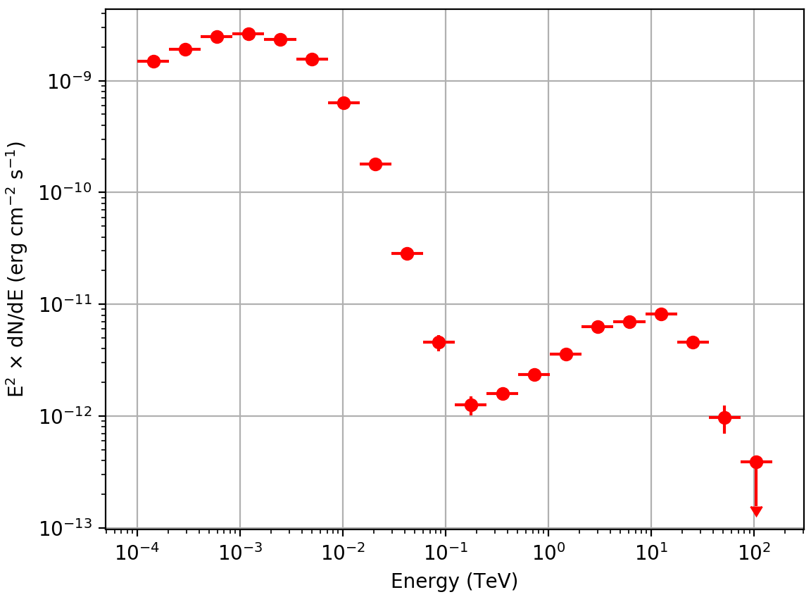
Vela spectrum derived using csspec from real Fermi-LAT and simulated CTA data

Note

The figure was created using the show_spectrum.py script that is located in the ctools example folder. The example script requires the matplotlib Python module for display. You may reproduce the plot by typing

$ $CTOOLS/share/examples/python/show_spectrum.py spectrum.fits