Joint analysis of H.E.S.S. and Fermi data

What you will learn

You will learn how to jointly analyse data from H.E.S.S. and Fermi.

In this tutorial you will learn how to jointly analyse data observed with H.E.S.S. and the Fermi-LAT. This follows the same procedure illustrated in this section.

Prepare Fermi-LAT data

For this tutorial you need to gather data for a source available in the H.E.S.S. public data release, the Crab nebula. The preparation of Fermi-LAT data can be adapted from this section. Get Source Class LAT data from the Crab in the energy range 50-1000 GeV. Apply a zenith angle cut at 105 deg. Then bin them on a 60x60 pixel grid with 0.05 deg step, and on a logarithmic energy grid with 15 bins from 50 GeV to 1 TeV, and calculate livetime cube, exposure map, and diffuse model source maps. The results shown here correspond to P8R3 LAT data covering the Fermi Mission Elapsed Time (MET) between 239557417 s and 565315205 s, analysed using the fermitools 1.0.1. To run the tutorial faster you can select a shorter dataset.

Prepare H.E.S.S. data

We will use the On/Off observations generated in this section.

Combining the observations

Now you have all the data and hand. You have to create an observation definition file to combine the data for an analysis:

<?xml version="1.0" standalone="no"?>
<observation_list title="observation library">
  <observation name="Crab" id="000001" instrument="LAT">
    <parameter name="CountsMap"    file="srcmaps.fits"/>
    <parameter name="ExposureMap"  file="expmap.fits"/>
    <parameter name="LiveTimeCube" file="ltcube.fits"/>
    <parameter name="IRF"          value="P8R3_SOURCE_V2"/>
  </observation>
  <observation name="Crab" id="000002" instrument="HESSOnOff" statistic="wstat">
    <parameter name="Pha_on" file="onoff_stacked_pha_on.fits" />
    <parameter name="Pha_off" file="onoff_stacked_pha_off.fits" />
    <parameter name="Arf" file="onoff_stacked_arf.fits" />
    <parameter name="Rmf" file="onoff_stacked_rmf.fits" />
  </observation>
</observation_list>

The instrument attribute distinguishes between the two instruments. Note how we have specified thet statistic attribute so that WSTAT will be used by all likelihood tools. Note how we are using different analysis methods for the LAT and H.E.S.S. data, that is binned and On/Off, respectively. Those are the standard analysis methods for each instrument, but you can use any other method for H.E.S.S. data, such as binned or unbinned. For H.E.S.S. you may choose another analysis method, such as unbinned or binned.

Fit a spectral model to the data

You have to define a model definition file that will be used to model the events for both observations. The model that will be used in this analysis is shown below:

<?xml version="1.0" standalone="no"?>
<source_library title="source library">
  <source type="PointSource" name="Crab">
    <spectrum type="LogParabola">
      <parameter name="Prefactor"   scale="1e-17" value="3.23"   min="1e-07" max="10000.0" free="1"/>
      <parameter name="Index"       scale="-1"    value="2.47" min="0.5"   max="+5.0"   free="1"/>
      <parameter name="Curvature"   scale="-1"    value="0.24"   min="-5.0"  max="+5.0"   free="1"/>
      <parameter name="PivotEnergy" scale="1e6"   value="1.0"     min="0.01"  max="1000.0" free="0"/>
    </spectrum>
    <spatialModel type="PointSource">
      <parameter name="RA"  scale="1.0" value="83.633" min="-360" max="360" free="0"/>
      <parameter name="DEC" scale="1.0" value="22.015" min="-90"  max="90"  free="0"/>
    </spatialModel>
  </source>
  <source type="DiffuseSource" name="Galactic_diffuse" instrument="LAT">
    <spectrum type="Constant">
      <parameter name="Normalization" scale="1.0" value="1.0" min="0.1" max="10.0" free="1"/>
    </spectrum>
    <spatialModel type="DiffuseMapCube" file="gll_iem_v07.fits">
      <parameter name="Normalization" scale="1.0" value="1.0" min="0.1" max="10.0" free="0"/>
    </spatialModel>
  </source>
  <source type="DiffuseSource" name="Isotropic_diffuse"  instrument="LAT">
    <spectrum type="FileFunction" file="iso_P8R2_SOURCE_V2_v1.txt">
      <parameter name="Normalization" scale="1.0" value="1.0" min="0.0" max="1000.0" free="0"/>
    </spectrum>
    <spatialModel type="DiffuseIsotropic">
      <parameter name="Value" scale="1.0" value="1.0" min="0.0" max="10.0" free="0"/>
    </spatialModel>
  </source>
</source_library>

The model contains a point source located at the position of the Crab with a log-parabola spectrum. It does not have any instrument attribute, which means that it applies to all instruments. In addition, the model contains two DiffuseSource components that are only applied for Fermi-LAT observations, which is indicated by their instrument="LAT" attribute. Both components model the diffuse background and are the same that were included in the generation of the source maps (the names need to coincide).

Now you can fit the model to the data using ctlike:

$ ctlike
Input event list, counts cube or observation definition XML file [] joint_observations.xml
Input model definition XML file [] joint_models.xml
Output model definition XML file [] joint_results.xml

The results are: prefactor (for 1 TeV pivot energy) (4.5±0.2)×10−11 photons cm−2 s−1 TeV−1, spectral index 2.42±0.04, and curvature -0.109±0.018. They are broadly consistent with results from published studies, e.g., MAGIC collaboration (2015). We have used an energy threshold of 50 GeV to avoid contamination from the Crab pulsar. The Fermi analysis can be extended to lower energies for example by selecting photons based on the pulsar phase.

Butterfly and SED

We can now generate the butterfly

$ ctbutterfly
Input event list, counts cube or observation definition XML file [events.fits] joint_observations.xml
Source of interest [Crab]
Input model definition XML file [$CTOOLS/share/models/crab.xml] joint_results.xml
Lower energy limit (TeV) [0.1] 0.05
Upper energy limit (TeV) [100.0]
Output ASCII file [butterfly.txt]

and spectral energy distribution (SED)

$ csspec
Input event list, counts cube, or observation definition XML file [joint_observations.xml]
Input model definition XML file [joint_results.xml]
Source name [Crab]
Spectrum generation method (SLICE|NODES|AUTO) [AUTO]
Algorithm for defining energy bins (FILE|LIN|LOG|POW) [LOG]
Start value for first energy bin in TeV [0.1] 0.05
Stop value for last energy bin in TeV [100.0]
Number of energy bins (1-200) [10] 15
Output spectrum file [spectrum.fits]

Below you can see the resulting butterfly and SED.

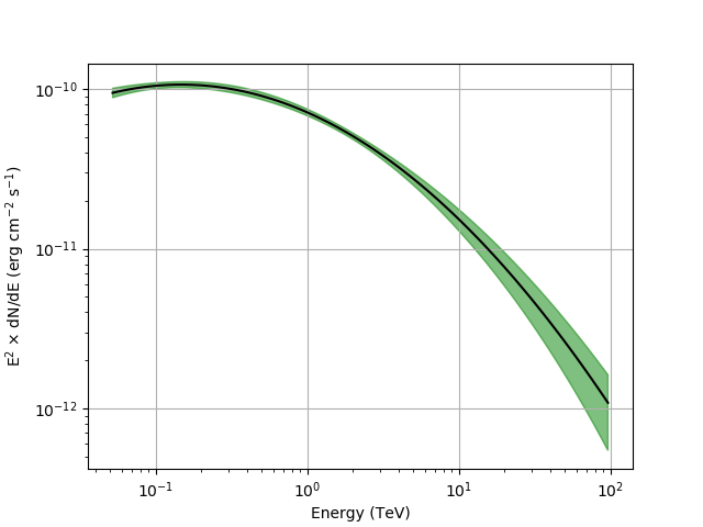
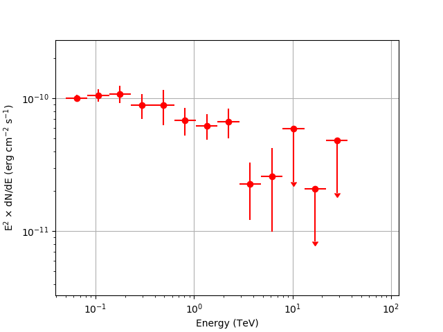
Spectral energy distribution of the Crab nebula from joint analysis of H.E.S.S. and Fermi data

Note

These figures were created by typing:

$ $CTOOLS/share/examples/python/show_butterfly.py butterfly.txt
$ $CTOOLS/share/examples/python/show_spectrum.py spectrum.fits

The SED is not shown above 40 TeV because the low counting statistics make the results uninteresting.