This temporal model component implements a light curve \(r(t)\)
\[M_{\rm temporal}(t) = N_0 \times r(t)\]
where
\(N_0\) = Normalization
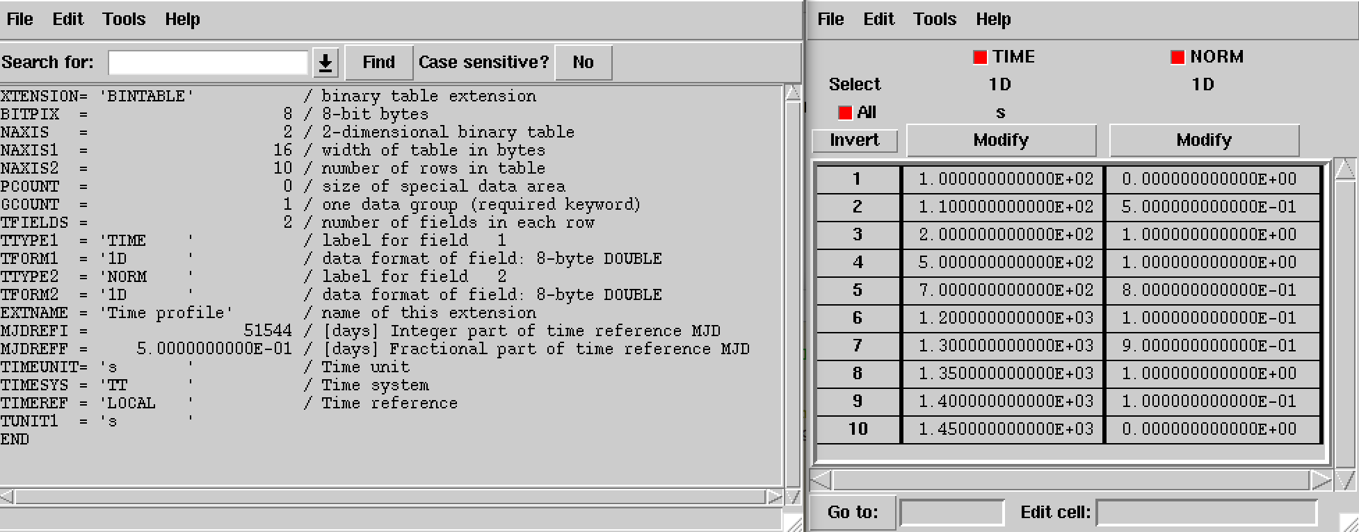
The light curve is defined by nodes in a FITS file that specify the relative
flux normalization as function of time (file model_temporal_lightcurve.fits
in the example above). The structure of the light curve FITS
file is shown in the figure below. The light curve is defined in the first
extension of the FITS file and consists of a binary table with the columns
TIME and NORM. Times in the TIME columns are given in seconds
and are counted with respect to a time reference that is defined in the
header of the binary table. Times need to be specified in ascending order.
The values in the NORM column specify \(r(t)\) at times \(t\),
and should be comprised between 0 and 1.
Fitting of light curves only makes sense for an unbinned maximum likelihood
analysis, since in a binned or stacked analysis the times of individual
events are dropped.
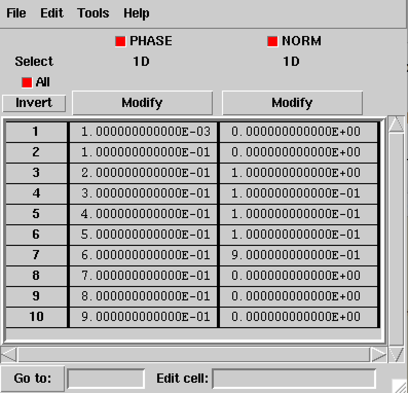
The phase curve is defined by nodes in a FITS file that specify the relative
flux normalization as function of phase (file model_temporal_phasecurve.fits
in the example above). The structure of the phase curve
FITS file is shown in the figure below. The phase curve is defined in the
first extension of the FITS file and consists of a binary table with the
columns PHASE and NORM. Phase values in the PHASE column need to
be comprised between 0 and 1 and need to be given in ascending order. The
values in the NORM column specify \(r(\Phi(t))\) at phases
\(\Phi(t)\), and should be comprised between 0 and 1.
By default, the NORM values are recomputed internally so that the
phase-averaged normalisation is one, i.e.
\[\int_0^1 r(\Phi) d\Phi = 1\]
In that case, the spectral component corresponds to the phase-averaged
spectrum. If the internal normalisation should be disabled the
normalize="0" attribute needs to be added to the temporal tag, i.e.
In that case the NORM values are directly multiplied with the spectral
component.
Warning
Fitting of phase curves only makes sense for an unbinned maximum likelihood
analysis, since in a binned or stacked analysis the times of individual
events are dropped.
Warning
Fitting of phase curve parameters may not properly work for pulsar
frequencies.