As gamma-ray events are rare, the counts cubes generated by ctbin will in general be sparsly populated, having many empty pixels, in particular at high energies. An alternative analysis technique consists of working directly on the event list without binning the events in a counts cube. You will see the benefit of such an analysis later once you re-run ctlike in unbinned mode.
For unbinned analysis you first have to define the data space region over which the analysis is done. This is similiar to the ctbin step for a binned analysis where you defined the size of the counts cube, the energy range, and the time interval. For unbinned analysis you have no such thing as a counts cube, but you have to define over which region of the data space the selected events are spread (because the ctools have to integrate over this region to compute the total number of predicted events in the data space that you analyse). Furthermore, you have to define what energy range is covered, and what time interval is spanned by the data. All this is done by the ctselect tool, which replaces the ctbin step in an unbinned analysis.
ctselect performs an event selection by choosing only events within a given region-of-interest (ROI), within a given energy band, and within a given time interval from the input event list. The ROI is a circular region on the sky, for which you define the centre (in celestial coordinates) and the radius. Such a circular ROI is sometimes also called an acceptance cone. The following example shows how to run ctselect:
$ ctselect
Input event list or observation definition XML file [events.fits]
RA for ROI centre (degrees) (0-360) [83.63]
Dec for ROI centre (degrees) (-90-90) [22.01]
Radius of ROI (degrees) (0-180) [3.0]
Start time (CTA MET in seconds) [0.0]
End time (CTA MET in seconds) [0.0]
Lower energy limit (TeV) [0.1]
Upper energy limit (TeV) [100.0]
Output event list or observation definition XML file [selected_events.fits]
ctselect takes the input event list events.fits, performs an event selection, and writes the selected event into the file selected_events.fits. The parameters it will query for are the centre of the ROI, the radius of the ROI, the start and stop time (in seconds), and the energy lower and upper limits (in TeV). The event selection information is also written as a set of data selection keywords to the output events file selected_events.fits, by respecting the same syntax that has been implemented for Fermi/LAT. The following image is a screen dump of the data selection keywords that have been written to the EVENTS header in the file selected_events.fits:
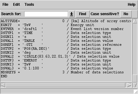
Data selection keywords
It is mandatory for an unbinned analysis that these data selection keywords exist in the FITS file. If they don’t exist, ctlike will not execute in unbinned mode.
Below some lines of the ctselect.log file that show the data selection part:
2016-06-29T16:20:10: +=================+
2016-06-29T16:20:10: | Event selection |
2016-06-29T16:20:10: +=================+
2016-06-29T16:20:10: === CTA observation ===
2016-06-29T16:20:10:  Input filename ............: events.fits
2016-06-29T16:20:10:  Event extension name ......: EVENTS
2016-06-29T16:20:10:  GTI extension name ........: GTI
2016-06-29T16:20:10:  Selected energy range .....: 0.1 - 100 TeV
2016-06-29T16:20:10:  Requested ROI .............: Centre(RA,DEC)=(83.63, 22.01) deg, Radius=3 deg
2016-06-29T16:20:10:  ROI of data ...............: Centre(RA,DEC)=(83.63, 22.01) deg, Radius=5 deg
2016-06-29T16:20:10:  Selected ROI ..............: Centre(RA,DEC)=(83.63, 22.01) deg, Radius=3 deg
2016-06-29T16:20:10:  cfitsio selection .........: ENERGY >= 0.10000000 && ENERGY <= 100.00000000 && ANGSEP(83.630000,22.010000,RA,DEC) <= 3.000000
2016-06-29T16:20:10:  FITS filename .............: /var/tmp/tmp.0.3aUIXn[EVENTS][ENERGY >= 0.10000000 && ENERGY <= 100.00000000 && ANGSEP(83.630000,22.010000,RA,DEC) <= 3.000000]
Note
ctobssim will also write data selection keywords in the event list FITS file, hence you can run ctlike directly on a FITS file produced by ctobssim. Any selection performed by ctselect needs to be fully enclosed within any previous selection, e.g. the ROI needs to be fully enclosed in the acceptance cone used for event simulation, the energy selection must be fully comprised in the range of simulated energies, the same applies for the temporal selection. ctselect will automatically adjust the selection parameters to guarantee full enclosure. To keep track of this adjustment, the ctselect log file quotes the requested selection, any existing selections, and the selection that was finally applied.
Note
ctselect may of course also be used for event selection prior to binned analysis, for example to select events for a given period in time. The WEIGHT extension of the counts cube will track the overlap between the ROI applied by ctselect and the counts cube, and this information will be transparently used in any further analysis to restrict the analysis on counts cube bins that contain data.
Now that you have selected the events of interest, you can run ctlike in unbinned mode. To do this you have to specify the selected event list instead of the counts cube:
$ ctlike
Input event list, counts cube or observation definition XML file [cntcube.fits] selected_events.fits
Calibration database [prod2]
Instrument response function [South_0.5h]
Input model XML file [$CTOOLS/share/models/crab.xml]
Output model XML file [crab_results.xml]
You will recognise that ctlike runs much faster in unbinned mode compared to binned mode. This is understandable as the selected event list contains only 21604 events, while the binned counts cube you used before had 200 x 200 x 20 = 800000 bins. As unbinned maximum likelihood fitting loops over the events (while binned maximum likelihood loops over the bins), there are much less operations to perform in unbinned than in binned mode (there is some additional overhead in unbinned mode that comes from integrating the models over the region of interest, yet this is negligible compared to the operations needed when looping over all pixels). So as long as you work with small event lists, unbinned mode is faster (this typically holds up to 50 hours of observing time for point sources). Unbinned ctlike should also be more precise as no binning is performed, hence there is no loss of information due to histogramming.
Below you see the corresponding output from the ctlike.log file. The fitted parameters are essentially identical to the ones found in binned mode. The slight difference with respect to the binned analysis may be explained by the different event sample that has been used for the analysis: while binned likelihood works on rectangular counts cubes, unbinned likelihood works on circular event selection regions. It is thus not possible to select exactly the same events for both analyses.
2016-06-29T16:24:44: +=================================+
2016-06-29T16:24:44: | Maximum likelihood optimisation |
2016-06-29T16:24:44: +=================================+
2016-06-29T16:24:45:  >Iteration   0: -logL=137562.094, Lambda=1.0e-03
2016-06-29T16:24:45:  >Iteration   1: -logL=137560.613, Lambda=1.0e-03, delta=1.481, max(|grad|)=2.548241 [Index:7]
2016-06-29T16:24:45:  >Iteration   2: -logL=137560.613, Lambda=1.0e-04, delta=0.001, max(|grad|)=0.027191 [Index:3]
...
2016-06-29T16:24:45: +=========================================+
2016-06-29T16:24:45: | Maximum likelihood optimisation results |
2016-06-29T16:24:45: +=========================================+
2016-06-29T16:24:45: === GOptimizerLM ===
2016-06-29T16:24:45:  Optimized function value ..: 137560.613
2016-06-29T16:24:45:  Absolute precision ........: 0.005
2016-06-29T16:24:45:  Acceptable value decrease .: 2
2016-06-29T16:24:45:  Optimization status .......: converged
2016-06-29T16:24:45:  Number of parameters ......: 10
2016-06-29T16:24:45:  Number of free parameters .: 4
2016-06-29T16:24:45:  Number of iterations ......: 2
2016-06-29T16:24:45:  Lambda ....................: 1e-05
2016-06-29T16:24:45:  Maximum log likelihood ....: -137560.613
2016-06-29T16:24:45:  Observed events  (Nobs) ...: 21604.000
2016-06-29T16:24:45:  Predicted events (Npred) ..: 21603.998 (Nobs - Npred = 0.00202556)
2016-06-29T16:24:45: === GModels ===
2016-06-29T16:24:45:  Number of models ..........: 2
2016-06-29T16:24:45:  Number of parameters ......: 10
2016-06-29T16:24:45: === GModelSky ===
2016-06-29T16:24:45:  Name ......................: Crab
2016-06-29T16:24:45:  Instruments ...............: all
2016-06-29T16:24:45:  Instrument scale factors ..: unity
2016-06-29T16:24:45:  Observation identifiers ...: all
2016-06-29T16:24:45:  Model type ................: PointSource
2016-06-29T16:24:45:  Model components ..........: "PointSource" * "PowerLaw" * "Constant"
2016-06-29T16:24:45:  Number of parameters ......: 6
2016-06-29T16:24:45:  Number of spatial par's ...: 2
2016-06-29T16:24:45:   RA .......................: 83.6331 [-360,360] deg (fixed,scale=1)
2016-06-29T16:24:45:   DEC ......................: 22.0145 [-90,90] deg (fixed,scale=1)
2016-06-29T16:24:45:  Number of spectral par's ..: 3
2016-06-29T16:24:45:   Prefactor ................: 5.828e-16 +/- 1.0219e-17 [1e-23,1e-13] ph/cm2/s/MeV (free,scale=1e-16,gradient)
2016-06-29T16:24:45:   Index ....................: -2.47546 +/- 0.0154751 [-0,-5]  (free,scale=-1,gradient)
2016-06-29T16:24:45:   PivotEnergy ..............: 300000 [10000,1e+09] MeV (fixed,scale=1e+06,gradient)
2016-06-29T16:24:45:  Number of temporal par's ..: 1
2016-06-29T16:24:45:   Normalization ............: 1 (relative value) (fixed,scale=1,gradient)
2016-06-29T16:24:45: === GCTAModelIrfBackground ===
2016-06-29T16:24:45:  Name ......................: CTABackgroundModel
2016-06-29T16:24:45:  Instruments ...............: CTA
2016-06-29T16:24:45:  Instrument scale factors ..: unity
2016-06-29T16:24:45:  Observation identifiers ...: all
2016-06-29T16:24:45:  Model type ................: "PowerLaw" * "Constant"
2016-06-29T16:24:45:  Number of parameters ......: 4
2016-06-29T16:24:45:  Number of spectral par's ..: 3
2016-06-29T16:24:45:   Prefactor ................: 1.0132 +/- 0.0138017 [0.001,1000] ph/cm2/s/MeV (free,scale=1,gradient)
2016-06-29T16:24:45:   Index ....................: 0.00653002 +/- 0.00831374 [-5,5]  (free,scale=1,gradient)
2016-06-29T16:24:45:   PivotEnergy ..............: 1e+06 [10000,1e+09] MeV (fixed,scale=1e+06,gradient)
2016-06-29T16:24:45:  Number of temporal par's ..: 1
2016-06-29T16:24:45:   Normalization ............: 1 (relative value) (fixed,scale=1,gradient)