To visualise the analysis results you can compute a butterfly diagram which shows the confidence band of the spectral fit using the ctbutterfly tool. The butterfly diagram is the envelope of all power law models that are within a given confidence limit compatible with the data. By default a confidence level of 68% is used, but the level can be adjusted using the hidden confidence parameter. ctbutterfly computes this envelope by evaluating for each energy the minimum and maximum intensity of all power law models that fall within the error ellipse of the prefactor and index parameters. The error ellipse is derived from the covariance matrix of a maximum likelihood fit.
The following example illustrates how you can use the ctbutterfly tool:
$ ctbutterfly
Input event list, counts cube or observation definition XML file [events.fits]
Calibration database [prod2]
Instrument response function [South_0.5h]
Input model XML file [$CTOOLS/share/models/crab.xml] crab_results.xml
Source of interest [Crab]
Start value for first energy bin in TeV [0.1]
Stop value for last energy bin in TeV [100.0]
Output ASCII file [butterfly.txt]
Now that you have computed the confidence band of the spectral fit and that you will have an ASCII file named butterfly.txt on disk you can visualise the butterfly using the script show_butterfly.py that is in the ctools example folder. You will need matplotlib on your system to make this work. To launch the script, type:
$CTOOLS/share/examples/python/show_butterfly.py butterfly.txt
This will result in a canvas which should look like the following:
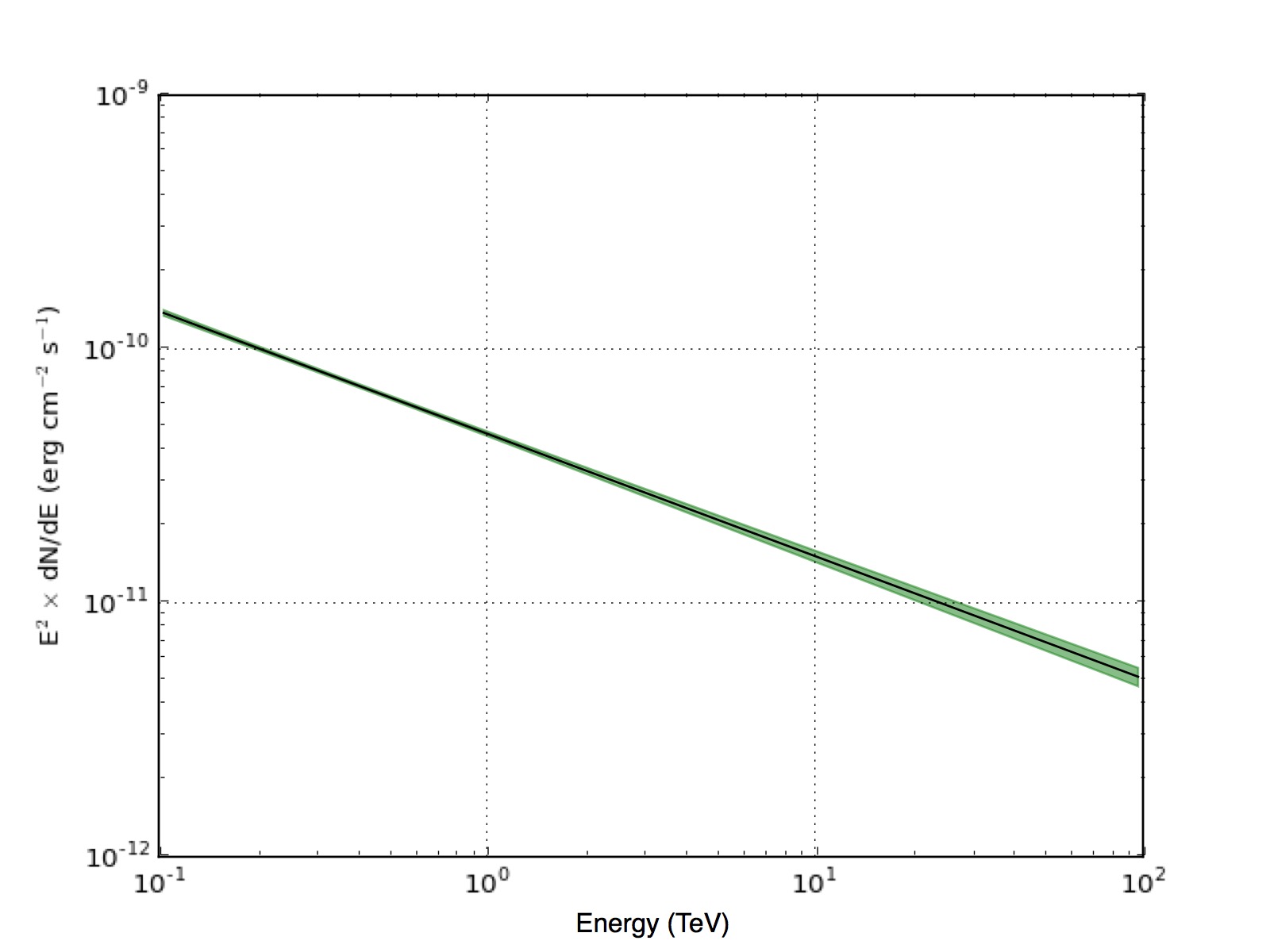
Confidence band of the power law fit