Generating your own event selection
What you will learn
You will learn how to use the GammaLib classes to generate your own data cubes and response functions for a COMPTEL analysis.
The data in the
HEASARC archive
comprises counts cubes for the standard COMPTEL energy ranges (0.75-1 MeV,
1-3 MeV, 3-10 MeV and 10-30 MeV) per viewing period. In case that you want
to analyse a different energy range, or that you want to perform a different
event selection, you need to create DRE, DRG, DRB and DRX
data and the corresponding IAQ response function yourself. You can do
this with GammaLib.
Let’s assume you want to make a 1.8 MeV line map of the Galactic centre.
You can use for this the data of the COMPTEL viewing period 16 in phase 1 of
the mission. Go to the
HEASARC archive
and download the EVP, TIM and OAD datasets. Once this is done,
create the following
observation definition file:
<?xml version="1.0" standalone="no"?>
<observation_list title="observation library">
  <observation name="GC" id="000160" instrument="COM">
    <parameter name="EVP" file="$COMDATA/phase01/vp0016_0/m28846_evp.fits"/>
    <parameter name="TIM" file="$COMDATA/phase01/vp0016_0/m11765_tim.fits"/>
    <parameter name="OAD" file="$COMDATA/phase01/vp0016_0/m20745_oad.fits"/>
    <parameter name="OAD" file="$COMDATA/phase01/vp0016_0/m20750_oad.fits"/>
    <parameter name="OAD" file="$COMDATA/phase01/vp0016_0/m20753_oad.fits"/>
    <parameter name="OAD" file="$COMDATA/phase01/vp0016_0/m20759_oad.fits"/>
    <parameter name="OAD" file="$COMDATA/phase01/vp0016_0/m20760_oad.fits"/>
    <parameter name="OAD" file="$COMDATA/phase01/vp0016_0/m20761_oad.fits"/>
    <parameter name="OAD" file="$COMDATA/phase01/vp0016_0/m20762_oad.fits"/>
    <parameter name="OAD" file="$COMDATA/phase01/vp0016_0/m20764_oad.fits"/>
    <parameter name="OAD" file="$COMDATA/phase01/vp0016_0/m20770_oad.fits"/>
    <parameter name="OAD" file="$COMDATA/phase01/vp0016_0/m20771_oad.fits"/>
    <parameter name="OAD" file="$COMDATA/phase01/vp0016_0/m20772_oad.fits"/>
    <parameter name="OAD" file="$COMDATA/phase01/vp0016_0/m20785_oad.fits"/>
    <parameter name="OAD" file="$COMDATA/phase01/vp0016_0/m20786_oad.fits"/>
    <parameter name="OAD" file="$COMDATA/phase01/vp0016_0/m20787_oad.fits"/>
    <parameter name="OAD" file="$COMDATA/phase01/vp0016_0/m20788_oad.fits"/>
    <parameter name="OAD" file="$COMDATA/phase01/vp0016_0/m20789_oad.fits"/>
  </observation>
</observation_list>
Note
There exist two formats for the
observation definition file
for COMPTEL data, one that describes the locations of the COMPTEL
data space cubes and response functions, and one that desribes
the location of an EVP event list, a TIM Good Time
Interval file, and an arbitrary number of OAD Orbit Aspect
Data files. In general there exists one OAD per day, while
there is one EVP event file and one TIM Good Time Interval
file per viewing period.
In the example above, the environment variable $COMDATA was set
to the root directory of the COMPTEL archive.
Now you are ready to generate the DRE, DRG, DRB, DRX and
IAQ datasets that you need for a ctools analysis of COMPTEL data.
This will take a few minutes. Start
Python
in your terminal and type the following:
# You need GammaLib, of course ;)
import gammalib

# Create sky map for the definition of the DRE and DRG data cubes
cube = gammalib.GSkyMap('TAN', 'GAL', 0.0, 20.0, 1.0, 1.0, 80, 80)

# Create sky map for the definition of the DRX exposure map
expo = gammalib.GSkyMap('CAR', 'GAL', 0.0, 0.0, 1.0, 1.0, 360, 180)

# Allocate DRE, DRG and DRX. DRE and DRG have a 3rd Phibar dimension, starting at 0.0 deg,
# with a binsize of 2.0 deg, and 25 Phibar layers.
dre = gammalib.GCOMDri(cube, 0.0, 2.0, 25)
drg = gammalib.GCOMDri(cube, 0.0, 2.0, 25)
drx = gammalib.GCOMDri(expo)

# Set DRE energy range to 1.7-1.9 MeV, DRG and DRX are energy independent
dre.ebounds(gammalib.GEbounds(gammalib.GEnergy(1.7, 'MeV'),
                              gammalib.GEnergy(1.9, 'MeV')))

# Load observation definition XML file 'obs.xml' (the file you created above)
obsdef = gammalib.GObservations('obs.xml')

# Compute DRE, DRG and DRX for the first observation in the XML file
dre.compute_dre(obsdef[0])
drg.compute_drg(obsdef[0])
drx.compute_drx(obsdef[0])

# Save DRE, DRG and DRX ('True' indicates to overwrite any existing file)
dre.save('dre.fits', True)
drg.save('drg.fits', True)
drx.save('drx.fits', True)

# Load DRE and DRG to generate a DRB background model cube
dre = gammalib.GCOMDri('dre.fits')
drb = gammalib.GCOMDri('drg.fits')

# Normalise DRB on the Phibar distribution of the DRE cube
npix = dre.nchi() * dre.npsi()
for k in range(dre.nphibar()):
    sum_dre = 0.0
    sum_drb = 0.0
    for i in range(npix):
        index    = i + k * npix
        sum_dre += dre[index]
        sum_drb += drb[index]
    if sum_drb > 0:
        for i in range(npix):
            index       = i + k * npix
            drb[index] *= sum_dre / sum_drb

# Save DRB
drb.save('drb.fits', True)

# Initialise IAQ that will hold the response function
iaq = gammalib.GCOMIaq(55.0, 1.0, 50.0, 2.0)

# Compute IAQ for a line energy of 1.809 MeV and an energy band of 1.7-1.9 MeV
iaq.set(gammalib.GEnergy(1.809, 'MeV'),
        gammalib.GEbounds(gammalib.GEnergy(1.7, 'MeV'),
                          gammalib.GEnergy(1.9, 'MeV')))

# Save IAQ and you are done
iaq.save('iaq.fits', True)
Now you have everything at hand to perform a COMPTEL maximum likelihood analysis. For that purpoe you need to gather all the datasets that you just created in a new observation definition file that should look as follows:
<?xml version="1.0" standalone="no"?>
<observation_list title="observation library">
  <observation name="GC" id="000160" instrument="COM">
    <parameter name="DRE" file="dre.fits"/>
    <parameter name="DRB" file="drb.fits"/>
    <parameter name="DRG" file="drg.fits"/>
    <parameter name="DRX" file="drx.fits"/>
    <parameter name="IAQ" value="iaq.fits"/>
  </observation>
</observation_list>
Warning
Be aware that the attribute for the IAQ parameter is value and
not file since the IAQ parameter is not necessarily a file
but can be also a response name of the calibration database.
Before doing a model fit you need a model. We included one in the ctools package
that you can find at $CTOOLS/share/models/comptel_howto_gc.xml. Here the
first few lines of this model:
<?xml version="1.0" encoding="UTF-8" standalone="no"?>
<source_library title="source library">
  <source name="GC" type="PointSource" tscalc="1">
    <spectrum type="Constant">
      <parameter name="Normalization" scale="1.0e-5" value="1.0"  min="-100.0" max="100.0" free="1"/>
    </spectrum>
    <spatialModel type="PointSource">
      <parameter name="RA"  scale="1.0" value="266.40" min="-360" max="360" free="0"/>
      <parameter name="DEC" scale="1.0" value="-28.94" min="-90"  max="90"  free="0"/>
    </spatialModel>
  </source>
  <source name="Background" type="DRBFitting" instrument="COM">
    <node>
      <parameter name="Phibar"        value="9"   scale="1" min="0" max="50"   free="0" />
      <parameter name="Normalization" value="1.0" scale="1" min="0" max="1000" free="1" />
    </node>
    ...
    <node>
      <parameter name="Phibar"        value="49"  scale="1" min="0" max="50"   free="0" />
      <parameter name="Normalization" value="1.0" scale="1" min="0" max="1000" free="1" />
    </node>
  </source>
</source_library>
This file contains a single point source at the position of the Galactic
Centre. The spectral model is a simple constant normalisation that will
return the gamma-ray line flux in units of
\({\rm photons}\,{\rm cm}^{-2}\,{\rm s}^{-1}\).
For the background we do a Phibar fitting of the DRB cube. Since the
first four layers of the DRE cube are empty we start the nodes at the
fifth layer which corresponds to a Phibar value of 9 degrees. There are
subsequent nodes spaced by 2 degrees (not shown) up to a Phibar value of
49 degrees.
Now it’s time for model fitting. You can produce for example a Test Statistic map of the region around the Galactic centre as follows:
$ cttsmap
Input event list, counts cube or observation definition XML file [events.fits] obs_dri.xml
Test source name [Crab] GC
Input model definition XML file [$CTOOLS/share/models/crab.xml] $CTOOLS/share/models/comptel_howto_gc.xml
Coordinate system (CEL - celestial, GAL - galactic) (CEL|GAL) [CEL] GAL
Projection method (AIT|AZP|CAR|GLS|MER|MOL|SFL|SIN|STG|TAN) [CAR]
First coordinate of image center in degrees (RA or galactic l) (0-360) [83.63] 0.0
Second coordinate of image center in degrees (DEC or galactic b) (-90-90) [22.01] 0.0
Image scale (in degrees/pixel) [0.02] 1.0
Size of the X axis in pixels [200] 50
Size of the Y axis in pixels [200] 30
Output Test Statistic map file [tsmap.fits]
Below is the resulting Test Statistic map that shows 1.8 MeV emission following the Galactic plane and peaking near the Galactic centre.
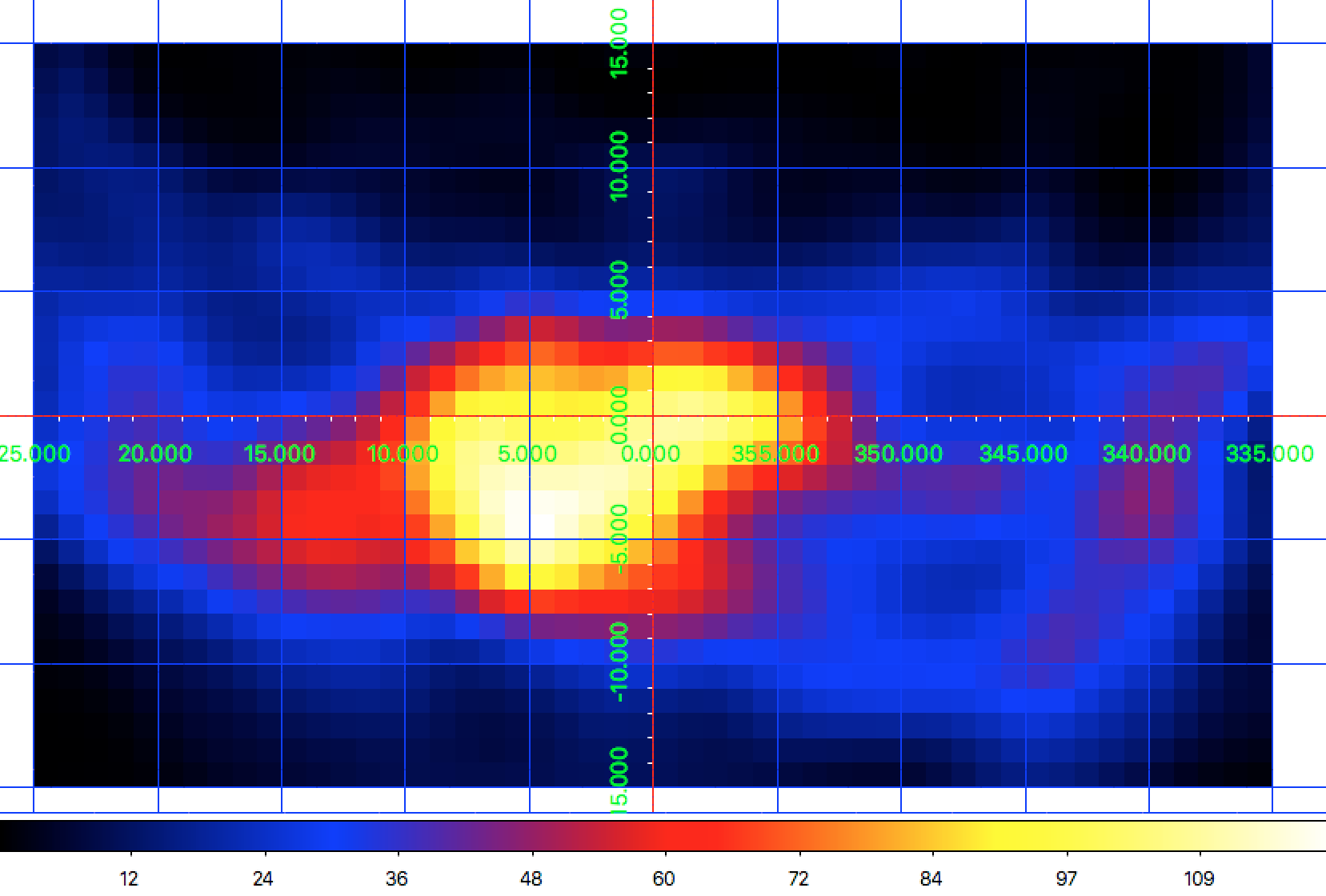
1.8 MeV Test Statistic map for COMPTEL viewing period 16 of the Galactic Centre
It is left to you as an exercise to extend this example. To get a better
statistics you may for example combine observations. For that purpose you
can add the DRI datasets of multiple observations into single DRE,
DRG, DRB and DRX datasets,
that’s the way how the COMPTEL analysis was done. You can however also leave
the DRI datasets separate and combine their description in the
observation definition file.
To combine for example the data of viewing periods 5, 7.5, 13, 16 and 27
the
observation definition file
should look like this:
<?xml version="1.0" standalone="no"?>
<observation_list title="observation library">
  <observation name="GC" id="000050" instrument="COM">
    <parameter name="DRE" file="dre_0050.fits"/>
    <parameter name="DRB" file="drb_0050.fits"/>
    <parameter name="DRG" file="drg_0050.fits"/>
    <parameter name="DRX" file="drx_0050.fits"/>
    <parameter name="IAQ" value="iaq.fits"/>
  </observation>
  <observation name="GC" id="000075" instrument="COM">
    <parameter name="DRE" file="dre_0075.fits"/>
    <parameter name="DRB" file="drb_0075.fits"/>
    <parameter name="DRG" file="drg_0075.fits"/>
    <parameter name="DRX" file="drx_0075.fits"/>
    <parameter name="IAQ" value="iaq.fits"/>
  </observation>
  <observation name="GC" id="000130" instrument="COM">
    <parameter name="DRE" file="dre_0130.fits"/>
    <parameter name="DRB" file="drb_0130.fits"/>
    <parameter name="DRG" file="drg_0130.fits"/>
    <parameter name="DRX" file="drx_0130.fits"/>
    <parameter name="IAQ" value="iaq.fits"/>
  </observation>
  <observation name="GC" id="000160" instrument="COM">
    <parameter name="DRE" file="dre_0160.fits"/>
    <parameter name="DRB" file="drb_0160.fits"/>
    <parameter name="DRG" file="drg_0160.fits"/>
    <parameter name="DRX" file="drx_0160.fits"/>
    <parameter name="IAQ" value="iaq.fits"/>
  </observation>
  <observation name="GC" id="000270" instrument="COM">
    <parameter name="DRE" file="dre_0270.fits"/>
    <parameter name="DRB" file="drb_0270.fits"/>
    <parameter name="DRG" file="drg_0270.fits"/>
    <parameter name="DRX" file="drx_0270.fits"/>
    <parameter name="IAQ" value="iaq.fits"/>
  </observation>
</observation_list>
The corresponding Test Statistic map is shown below.

1.8 MeV Test Statistic map for COMPTEL viewing periods 5, 7.5, 13, 16 and 27 of the Galactic Centre