Performing an unbinned analysis
In this tutorial you will learn to fit a parametric model to the event data (unbinned fit) and how to inspect the fit residuals
Now you are ready to fit the models for the source and the background to the data.
We start by importing gammalib, ctools, and cscripts.
In [1]:
import gammalib
import ctools
import cscripts
We will also use matplotlib to display the results.
In [2]:
%matplotlib inline
import matplotlib.pyplot as plt
Finally we add to our path the directory containing the example plotting scripts provided with the ctools installation.
In [3]:
import sys
import os
sys.path.append(os.environ['CTOOLS']+'/share/examples/python/')
Preparing the model
First, we will merge the two models we derived in the previous tutorials for source and background.
In [4]:
srcmodel = 'crab.xml'
bkgmodel = 'bkgmodel.xml'
models   = gammalib.GModels()
for inmodels in [srcmodel,bkgmodel]:
    for model in gammalib.GModels(inmodels):
        models.append(model)
print(models)
=== GModels ===
 Number of models ..........: 5
 Number of parameters ......: 86
=== GModelSky ===
 Name ......................: Src001
 Instruments ...............: all
 Observation identifiers ...: all
 Model type ................: PointSource
 Model components ..........: "PointSource" * "PowerLaw" * "Constant"
 Number of parameters ......: 6
 Number of spatial par's ...: 2
  RA .......................: 83.6192131308071 +/- 0 deg (free,scale=1)
  DEC ......................: 22.0199996472185 +/- 0 deg (free,scale=1)
 Number of spectral par's ..: 3
  Prefactor ................: 5.7e-18 +/- 0 [0,infty[ ph/cm2/s/MeV (free,scale=5.7e-18,gradient)
  Index ....................: -2.48 +/- 0 [10,-10]  (free,scale=-2.48,gradient)
  PivotEnergy ..............: 300000 MeV (fixed,scale=300000,gradient)
 Number of temporal par's ..: 1
  Normalization ............: 1 (relative value) (fixed,scale=1,gradient)
 Number of scale par's .....: 0
=== GCTAModelBackground ===
 Name ......................: Background_023523
 Instruments ...............: HESS
 Observation identifiers ...: 023523
 Model type ................: CTABackground
 Model components ..........: "Multiplicative" * "NodeFunction" * "Constant"
 Number of parameters ......: 20
 Number of spatial par's ...: 3
  1:Normalization ..........: 1 [0.001,1000]  (fixed,scale=1,gradient)
  2:Grad_DETX ..............: 0.0881748792818854 +/- 0.0222611841905954 deg^-1 (free,scale=1,gradient)
  2:Grad_DETY ..............: -0.000701218995455618 +/- 0.0227202811076142 deg^-1 (free,scale=1,gradient)
 Number of spectral par's ..: 16
  Energy0 ..................: 700000 [7e-05,infty[ MeV (fixed,scale=700000)
  Intensity0 ...............: 0.00167503068442416 +/- 0.000204995398027476 [1.00182541969977e-13,infty[ ph/cm2/s/MeV (free,scale=0.00100182541969977,gradient)
  Energy1 ..................: 1197413.67463685 [0.000119741367463685,infty[ MeV (fixed,scale=1197413.67463685)
  Intensity1 ...............: 0.000275120588592054 +/- 1.41610992132859e-05 [3.21240099713853e-14,infty[ ph/cm2/s/MeV (free,scale=0.000321240099713853,gradient)
  Energy2 ..................: 2048285.01172474 [0.000204828501172474,infty[ MeV (fixed,scale=2048285.01172474)
  Intensity2 ...............: 0.000102369982797547 +/- 5.87189405970882e-06 [1.03007170346199e-14,infty[ ph/cm2/s/MeV (free,scale=0.000103007170346199,gradient)
  Energy3 ..................: 3503777.83227556 [0.000350377783227556,infty[ MeV (fixed,scale=3503777.83227556)
  Intensity3 ...............: 3.43310169853447e-05 +/- 2.52595458342912e-06 [3.30297405342054e-15,infty[ ph/cm2/s/MeV (free,scale=3.30297405342054e-05,gradient)
  Energy4 ..................: 5993530.69893743 [0.000599353069893743,infty[ MeV (fixed,scale=5993530.69893743)
  Intensity4 ...............: 1.04184963555313e-05 +/- 1.01064863096553e-06 [1.05911438600856e-15,infty[ ph/cm2/s/MeV (free,scale=1.05911438600856e-05,gradient)
  Energy5 ..................: 10252479.454662 [0.0010252479454662,infty[ MeV (fixed,scale=10252479.454662)
  Intensity5 ...............: 4.1837003769505e-06 +/- 5.25942224806527e-07 [3.39610080039421e-16,infty[ ph/cm2/s/MeV (free,scale=3.39610080039421e-06,gradient)
  Energy6 ..................: 17537798.7113509 [0.00175377987113509,infty[ MeV (fixed,scale=17537798.7113509)
  Intensity6 ...............: 8.6658971981008e-07 +/- 1.76584928413557e-07 [1.08897592165697e-16,infty[ ph/cm2/s/MeV (free,scale=1.08897592165697e-06,gradient)
  Energy7 ..................: 30000000 [0.003,infty[ MeV (fixed,scale=30000000)
  Intensity7 ...............: 3.41087754372141e-07 +/- 1.23894301613722e-07 [3.49185323889972e-17,infty[ ph/cm2/s/MeV (free,scale=3.49185323889972e-07,gradient)
 Number of temporal par's ..: 1
  Normalization ............: 1 (relative value) (fixed,scale=1,gradient)
=== GCTAModelBackground ===
 Name ......................: Background_023526
 Instruments ...............: HESS
 Observation identifiers ...: 023526
 Model type ................: CTABackground
 Model components ..........: "Multiplicative" * "NodeFunction" * "Constant"
 Number of parameters ......: 20
 Number of spatial par's ...: 3
  1:Normalization ..........: 1 [0.001,1000]  (fixed,scale=1,gradient)
  2:Grad_DETX ..............: 0.0153166143265463 +/- 0.0215144304488992 deg^-1 (free,scale=1,gradient)
  2:Grad_DETY ..............: -0.00908019181469828 +/- 0.0213167666197536 deg^-1 (free,scale=1,gradient)
 Number of spectral par's ..: 16
  Energy0 ..................: 700000 [7e-05,infty[ MeV (fixed,scale=700000)
  Intensity0 ...............: 0.00126074399446221 +/- 6.18948752992e-05 [9.62519069451052e-14,infty[ ph/cm2/s/MeV (free,scale=0.000962519069451052,gradient)
  Energy1 ..................: 1197413.67463685 [0.000119741367463685,infty[ MeV (fixed,scale=1197413.67463685)
  Intensity1 ...............: 0.000220109488746193 +/- 1.10099106908638e-05 [2.95441986174209e-14,infty[ ph/cm2/s/MeV (free,scale=0.000295441986174209,gradient)
  Energy2 ..................: 2048285.01172474 [0.000204828501172474,infty[ MeV (fixed,scale=2048285.01172474)
  Intensity2 ...............: 0.000104377151461511 +/- 6.26567390995899e-06 [9.068492247571e-15,infty[ ph/cm2/s/MeV (free,scale=9.068492247571e-05,gradient)
  Energy3 ..................: 3503777.83227556 [0.000350377783227556,infty[ MeV (fixed,scale=3503777.83227556)
  Intensity3 ...............: 2.68164289254463e-05 +/- 2.2601490434718e-06 [2.78354314866283e-15,infty[ ph/cm2/s/MeV (free,scale=2.78354314866283e-05,gradient)
  Energy4 ..................: 5993530.69893743 [0.000599353069893743,infty[ MeV (fixed,scale=5993530.69893743)
  Intensity4 ...............: 8.96128027251196e-06 +/- 9.61601396204211e-07 [8.54399193266454e-16,infty[ ph/cm2/s/MeV (free,scale=8.54399193266454e-06,gradient)
  Energy5 ..................: 10252479.454662 [0.0010252479454662,infty[ MeV (fixed,scale=10252479.454662)
  Intensity5 ...............: 3.14829249162658e-06 +/- 4.37081753413707e-07 [2.62254954375342e-16,infty[ ph/cm2/s/MeV (free,scale=2.62254954375342e-06,gradient)
  Energy6 ..................: 17537798.7113509 [0.00175377987113509,infty[ MeV (fixed,scale=17537798.7113509)
  Intensity6 ...............: 6.09624701513041e-07 +/- 1.43872314987655e-07 [8.04982748537824e-17,infty[ ph/cm2/s/MeV (free,scale=8.04982748537824e-07,gradient)
  Energy7 ..................: 30000000 [0.003,infty[ MeV (fixed,scale=30000000)
  Intensity7 ...............: 3.44982419809933e-07 +/- 1.26076763285202e-07 [2.4708674312253e-17,infty[ ph/cm2/s/MeV (free,scale=2.4708674312253e-07,gradient)
 Number of temporal par's ..: 1
  Normalization ............: 1 (relative value) (fixed,scale=1,gradient)
=== GCTAModelBackground ===
 Name ......................: Background_023559
 Instruments ...............: HESS
 Observation identifiers ...: 023559
 Model type ................: CTABackground
 Model components ..........: "Multiplicative" * "NodeFunction" * "Constant"
 Number of parameters ......: 20
 Number of spatial par's ...: 3
  1:Normalization ..........: 1 [0.001,1000]  (fixed,scale=1,gradient)
  2:Grad_DETX ..............: 0.018749400342 +/- 0.0217067733288596 deg^-1 (free,scale=1,gradient)
  2:Grad_DETY ..............: -0.126640342510319 +/- 0.020455126417247 deg^-1 (free,scale=1,gradient)
 Number of spectral par's ..: 16
  Energy0 ..................: 700000 [7e-05,infty[ MeV (fixed,scale=700000)
  Intensity0 ...............: 0.00109294743570479 +/- 5.37668986080239e-05 [8.7418891142236e-14,infty[ ph/cm2/s/MeV (free,scale=0.00087418891142236,gradient)
  Energy1 ..................: 1197413.67463685 [0.000119741367463685,infty[ MeV (fixed,scale=1197413.67463685)
  Intensity1 ...............: 0.000220103906688583 +/- 1.10283166290448e-05 [2.69181956755491e-14,infty[ ph/cm2/s/MeV (free,scale=0.000269181956755491,gradient)
  Energy2 ..................: 2048285.01172474 [0.000204828501172474,infty[ MeV (fixed,scale=2048285.01172474)
  Intensity2 ...............: 8.06623852687504e-05 +/- 5.23872750218462e-06 [8.28870337932099e-15,infty[ ph/cm2/s/MeV (free,scale=8.28870337932099e-05,gradient)
  Energy3 ..................: 3503777.83227556 [0.000350377783227556,infty[ MeV (fixed,scale=3503777.83227556)
  Intensity3 ...............: 2.85428972580395e-05 +/- 2.37266748207121e-06 [2.55227373106486e-15,infty[ ph/cm2/s/MeV (free,scale=2.55227373106486e-05,gradient)
  Energy4 ..................: 5993530.69893743 [0.000599353069893743,infty[ MeV (fixed,scale=5993530.69893743)
  Intensity4 ...............: 6.46456658892385e-06 +/- 7.36558401693409e-07 [7.85901111449516e-16,infty[ ph/cm2/s/MeV (free,scale=7.85901111449516e-06,gradient)
  Energy5 ..................: 10252479.454662 [0.0010252479454662,infty[ MeV (fixed,scale=10252479.454662)
  Intensity5 ...............: 3.20506991372933e-06 +/- 4.41036712274814e-07 [2.4199620497598e-16,infty[ ph/cm2/s/MeV (free,scale=2.4199620497598e-06,gradient)
  Energy6 ..................: 17537798.7113509 [0.00175377987113509,infty[ MeV (fixed,scale=17537798.7113509)
  Intensity6 ...............: 9.17351299053318e-07 +/- 2.02856047440946e-07 [7.45159440158635e-17,infty[ ph/cm2/s/MeV (free,scale=7.45159440158635e-07,gradient)
  Energy7 ..................: 30000000 [0.003,infty[ MeV (fixed,scale=30000000)
  Intensity7 ...............: 1.93348643577948e-07 +/- 9.48901838749967e-08 [2.29450949990163e-17,infty[ ph/cm2/s/MeV (free,scale=2.29450949990163e-07,gradient)
 Number of temporal par's ..: 1
  Normalization ............: 1 (relative value) (fixed,scale=1,gradient)
=== GCTAModelBackground ===
 Name ......................: Background_023592
 Instruments ...............: HESS
 Observation identifiers ...: 023592
 Model type ................: CTABackground
 Model components ..........: "Multiplicative" * "NodeFunction" * "Constant"
 Number of parameters ......: 20
 Number of spatial par's ...: 3
  1:Normalization ..........: 1 [0.001,1000]  (fixed,scale=1,gradient)
  2:Grad_DETX ..............: 0.0290076925442388 +/- 0.0231627042594752 deg^-1 (free,scale=1,gradient)
  2:Grad_DETY ..............: 0.165459453396994 +/- 0.0212165299830029 deg^-1 (free,scale=1,gradient)
 Number of spectral par's ..: 16
  Energy0 ..................: 700000 [7e-05,infty[ MeV (fixed,scale=700000)
  Intensity0 ...............: 0.00173543806725313 +/- 0.000221842434989178 [9.64800822522881e-14,infty[ ph/cm2/s/MeV (free,scale=0.000964800822522881,gradient)
  Energy1 ..................: 1197413.67463685 [0.000119741367463685,infty[ MeV (fixed,scale=1197413.67463685)
  Intensity1 ...............: 0.000247432426542881 +/- 1.35075275068334e-05 [3.05783271724063e-14,infty[ ph/cm2/s/MeV (free,scale=0.000305783271724063,gradient)
  Energy2 ..................: 2048285.01172474 [0.000204828501172474,infty[ MeV (fixed,scale=2048285.01172474)
  Intensity2 ...............: 0.000102349095137416 +/- 6.00669028431716e-06 [9.6914727976462e-15,infty[ ph/cm2/s/MeV (free,scale=9.6914727976462e-05,gradient)
  Energy3 ..................: 3503777.83227556 [0.000350377783227556,infty[ MeV (fixed,scale=3503777.83227556)
  Intensity3 ...............: 3.39523135381865e-05 +/- 2.54888013407308e-06 [3.07160834724385e-15,infty[ ph/cm2/s/MeV (free,scale=3.07160834724385e-05,gradient)
  Energy4 ..................: 5993530.69893743 [0.000599353069893743,infty[ MeV (fixed,scale=5993530.69893743)
  Intensity4 ...............: 9.09839000917866e-06 +/- 9.25509371718351e-07 [9.735133179293e-16,infty[ ph/cm2/s/MeV (free,scale=9.735133179293e-06,gradient)
  Energy5 ..................: 10252479.454662 [0.0010252479454662,infty[ MeV (fixed,scale=10252479.454662)
  Intensity5 ...............: 3.01613230297962e-06 +/- 4.11382625961797e-07 [3.08544603688196e-16,infty[ ph/cm2/s/MeV (free,scale=3.08544603688196e-06,gradient)
  Energy6 ..................: 17537798.7113509 [0.00175377987113509,infty[ MeV (fixed,scale=17537798.7113509)
  Intensity6 ...............: 9.30049222211062e-07 +/- 1.86843120695054e-07 [9.77899025229569e-17,infty[ ph/cm2/s/MeV (free,scale=9.77899025229569e-07,gradient)
  Energy7 ..................: 30000000 [0.003,infty[ MeV (fixed,scale=30000000)
  Intensity7 ...............: 3.98006363733031e-07 +/- 1.41569683967725e-07 [3.09934606573553e-17,infty[ ph/cm2/s/MeV (free,scale=3.09934606573553e-07,gradient)
 Number of temporal par's ..: 1
  Normalization ............: 1 (relative value) (fixed,scale=1,gradient)
Note how the source found by cssrcdetect was named Src001. We will call it Crab instead. Also, spectral parameters are set to default values, but you should make sure they are appropriate so that the model fit runs seamlessly. In this case it is best to set the value of the pivot energy for the Crab within our energy range (> 0.66 TeV). We will set it to 1 TeV.
In [5]:
models['Src001'].name('Crab')
models['Crab']['PivotEnergy'].value(1.e6)
We will save this model to disk for later use.
In [6]:
modelfile = 'crab_models.xml'
models.save(modelfile)
Fitting the model to the data
The model fit is performed by ctlike. We will use the previously selected events.
In [7]:
obsfile = 'obs_crab_selected.xml'
like    = ctools.ctlike()
like['inobs']   = obsfile
like['inmodel'] = modelfile
like.run()
We can now look at the results from the optimisation and the fitted model.
In [8]:
print(like.opt())
print(like.obs().models()['Crab'])
=== GOptimizerLM ===
 Optimized function value ..: 98167.993
 Absolute precision ........: 0.005
 Acceptable value decrease .: 2
 Optimization status .......: converged
 Number of parameters ......: 86
 Number of free parameters .: 44
 Number of iterations ......: 28
 Lambda ....................: 0.1
=== GModelSky ===
 Name ......................: Crab
 Instruments ...............: all
 Observation identifiers ...: all
 Model type ................: PointSource
 Model components ..........: "PointSource" * "PowerLaw" * "Constant"
 Number of parameters ......: 6
 Number of spatial par's ...: 2
  RA .......................: 83.6231161425766 +/- 0.00240718177620446 deg (free,scale=1)
  DEC ......................: 22.0247773403131 +/- 0.00218186675985154 deg (free,scale=1)
 Number of spectral par's ..: 3
  Prefactor ................: 4.80653958161532e-17 +/- 2.64950884427518e-18 [0,infty[ ph/cm2/s/MeV (free,scale=5.7e-18,gradient)
  Index ....................: -2.68230589724908 +/- 0.0650730512302727 [10,-10]  (free,scale=-2.48,gradient)
  PivotEnergy ..............: 999999.999999999 MeV (fixed,scale=300000,gradient)
 Number of temporal par's ..: 1
  Normalization ............: 1 (relative value) (fixed,scale=1,gradient)
 Number of scale par's .....: 0
The statistical 1-sigma positional uncertainty corresponds to 0.12 arcmin. Systematic uncertainties are not computed. The fitted position can be compared to the values of 83.629±0.005 degrees in Right Ascension and 22.012±0.001 degrees in Declination reported in Holler et al. (2017).
According to SIMBAD, the Crab nebula is situated at a Right Ascension of 83.633 degrees and a Declination of 22.015 degrees, which is 0.013 degrees (0.82 arcmin) away from the fitted position.
The intensity at 1 TeV of the Crab was fitted to (4.89±0.27)×10−11 photons cm−2 s−1 TeV−1 the spectral index of the power law is −2.70±0.07. This can be compared to the values of (3.45±0.05)×10−11 photons cm−2 s−1 TeV−1 and −2.63±0.01 reported in Aharonian et al. (2006), A&A, 457, 899 (note that the datasets, calibrations etc. used in our analysis are not the same as in that paper).
In the ctlike run above the energy dispersion, which relates the true photon energies to the energies of the reconstructed events, was not taken into account. By default energy dispersion usage is disabled since it involves an extra dimension in the data analysis which slows down the computations. We can run accounting for energy dispersion to compare the results.
In [9]:
like['edisp'] = True
like.run()
In [10]:
print(like.opt())
print(like.obs().models()['Crab'])
=== GOptimizerLM ===
 Optimized function value ..: 98168.820
 Absolute precision ........: 0.005
 Acceptable value decrease .: 2
 Optimization status .......: converged
 Number of parameters ......: 86
 Number of free parameters .: 44
 Number of iterations ......: 13
 Lambda ....................: 1
=== GModelSky ===
 Name ......................: Crab
 Instruments ...............: all
 Observation identifiers ...: all
 Model type ................: PointSource
 Model components ..........: "PointSource" * "PowerLaw" * "Constant"
 Number of parameters ......: 6
 Number of spatial par's ...: 2
  RA .......................: 83.6217013908939 +/- 0.00262422672788241 deg (free,scale=1)
  DEC ......................: 22.0244582493434 +/- 0.00238660922515514 deg (free,scale=1)
 Number of spectral par's ..: 3
  Prefactor ................: 4.56725958702027e-17 +/- 2.41200684919881e-18 [0,infty[ ph/cm2/s/MeV (free,scale=5.7e-18,gradient)
  Index ....................: -2.66140151299329 +/- 0.0671763204868478 [10,-10]  (free,scale=-2.48,gradient)
  PivotEnergy ..............: 999999.999999999 MeV (fixed,scale=300000,gradient)
 Number of temporal par's ..: 1
  Normalization ............: 1 (relative value) (fixed,scale=1,gradient)
 Number of scale par's .....: 0
You can verify that the results are broadly consistents with those obtained ignoring the energy dispersion.
Inspecting the fit residuals
Following a model fit, you should always inspect the fit residuals. First let’s inspect the spectral residuals. You can do this using the csresspec script.
In [11]:
residuals = 'residuals.fits'
resspec   = cscripts.csresspec(like.obs())
resspec['stack']       = True
resspec['components']  = True
resspec['ebinalg']     = 'LOG'
resspec['emin']        = 0.66
resspec['emax']        = 100.
resspec['enumbins']    = 20
resspec['proj']        = 'CAR'
resspec['coordsys']    = 'CEL'
resspec['xref']        = 83.63
resspec['yref']        = 22.01
resspec['binsz']       = 0.02
resspec['nxpix']       = 200
resspec['nypix']       = 200
resspec['algorithm']   = 'SIGNIFICANCE'
resspec['outfile']     = residuals
resspec.execute()
from show_residuals import plot_residuals
plot_residuals(residuals,'',0)
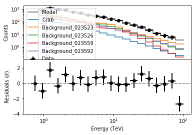
The spectral fit looks satisfactory. Finally you should also inspect the spatial residuals. You do this using the csresmap script.
In [12]:
resmap = cscripts.csresmap(like.obs())
resmap['emin']      = 0.66
resmap['emax']      = 100.0
resmap['proj']      = 'CAR'
resmap['coordsys']  = 'CEL'
resmap['xref']      = 83.63
resmap['yref']      = 22.01
resmap['binsz']     = 0.02
resmap['nxpix']     = 200
resmap['nypix']     = 200
resmap['algorithm'] = 'SUBDIV'
resmap.run()
We will inspect the residual map with a slight smoothing to suppress statistical fluctuations.
In [13]:
resmap._resmap.smooth('GAUSSIAN',0.1)
ax  = plt.subplot()
plt.imshow(resmap._resmap.array(),origin='lower',
            cmap='bwr',vmin=-1,vmax=1,
            extent=[83.63+0.02*200,83.63-0.02*200,22.01-0.02*200,22.01+0.02*200])
            # Boundaries of the coord grid
ax.set_xlabel('R.A. (deg)')
ax.set_ylabel('Dec (deg)')
cbar = plt.colorbar()
cbar.set_label('Residuals/Total Counts')
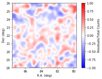
The residuals look flat across the field analysed.