Prepare Fermi-LAT data
What you will learn
You will learn how to prepare Fermi-LAT data for an analysis with ctools.
You will find more information about the Fermi-LAT software and data analysis at the Fermi Science Support Center (FSSC) web site.
Prerequisits
The following sections assume that you have properly installed the Fermi-LAT Science Tools. The Fermi-LAT Science Tools can be downloaded from the Fermi Science Support Center (FSSC).
Get data from the Fermi-LAT data server
Start with requesting the data you are interested in from the Fermi-LAT Data server. As example the figure below shows a request for data around the Vela pulsar.
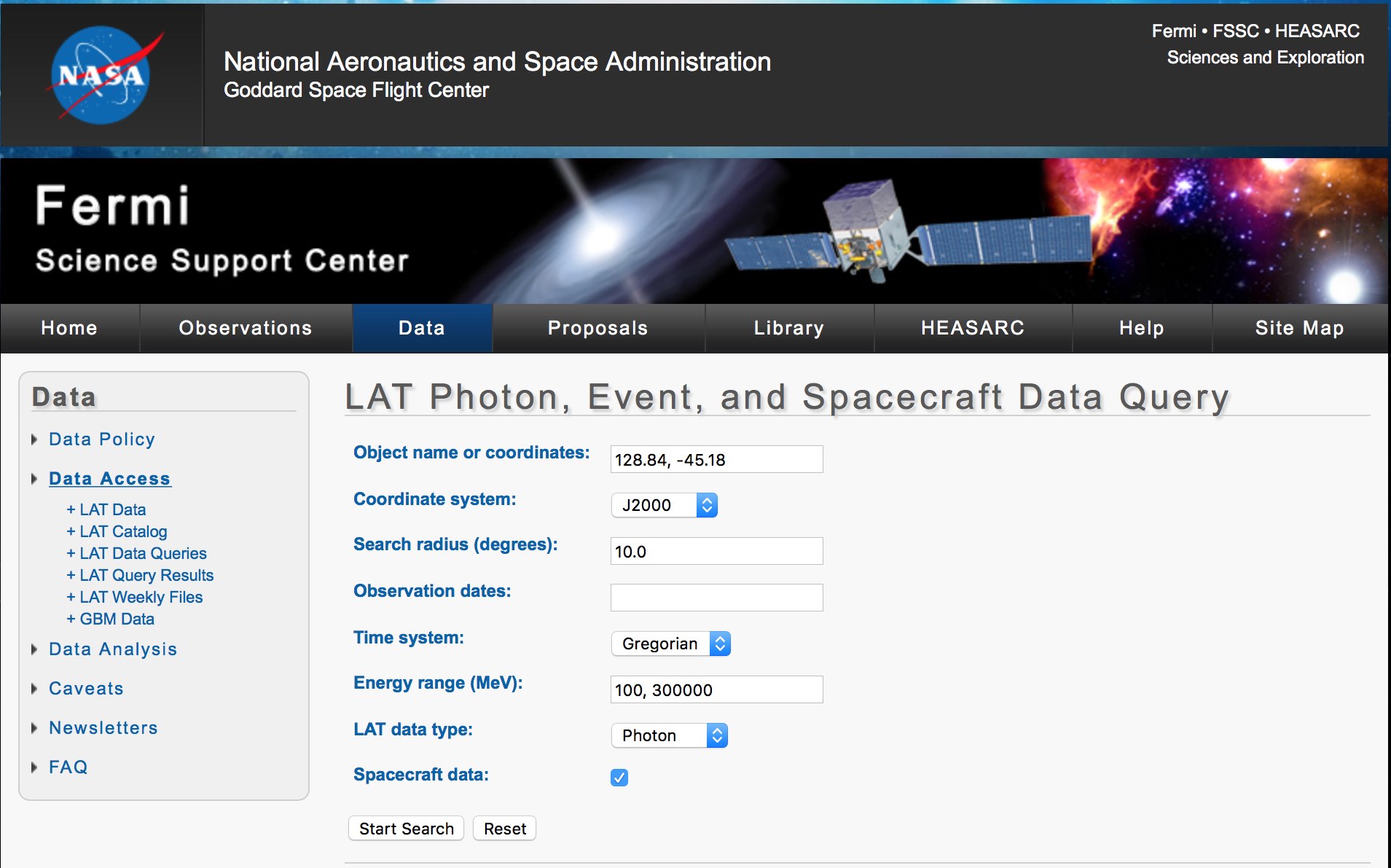
Fermi-LAT data server interface
After submitting the request you will get information of how to retrieve the data:
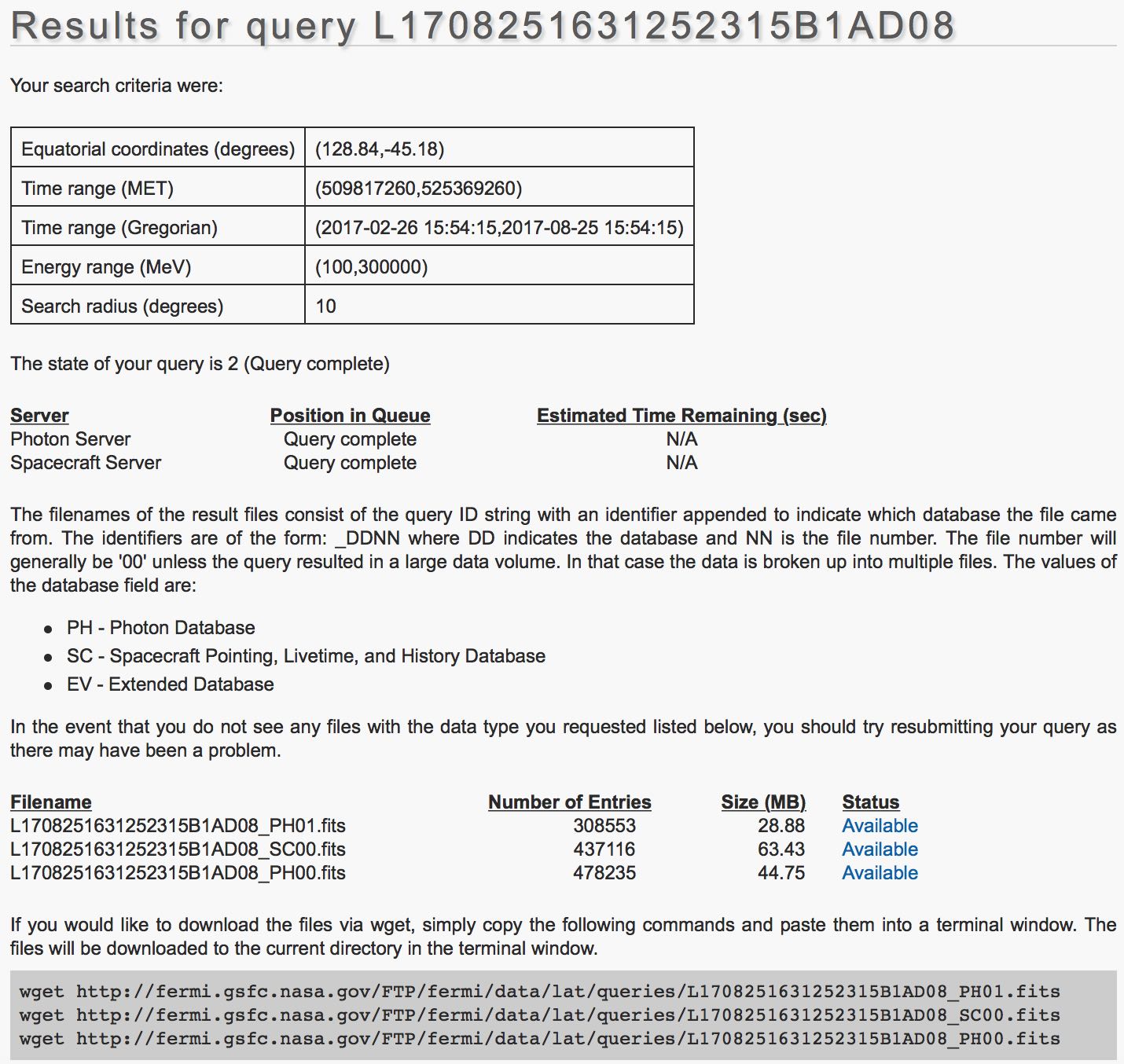
Fermi-LAT data retrieval information
Now you download the data using the wget tool. At the same time of
downloading the data you should also download the input files for the diffuse
galactic and extragalactic model components. In the current example the
following files were downloaded:
$ wget http://fermi.gsfc.nasa.gov/FTP/fermi/data/lat/queries/L1708251631252315B1AD08_SC00.fits
$ wget http://fermi.gsfc.nasa.gov/FTP/fermi/data/lat/queries/L1708251631252315B1AD08_PH00.fits
$ wget http://fermi.gsfc.nasa.gov/FTP/fermi/data/lat/queries/L1708251631252315B1AD08_PH01.fits
$ wget https://fermi.gsfc.nasa.gov/ssc/data/analysis/software/aux/gll_iem_v06.fits
$ wget https://fermi.gsfc.nasa.gov/ssc/data/analysis/software/aux/iso_P8R2_SOURCE_V6_v06.txt
Warning
In the current example data within a radius of only 10 degrees around the source of interest were selected. This was mainly for getting a small data set. The Fermi Science Support Center (FSSC) recommends to use larger regions for the Fermi-LAT data analysis.
Data preparation
First you need to combine the event lists into a single file. At the same
time you will select the region of interest for the analysis. You do this
using the gtselect tool:
$ ls *_PH* > events.txt
$ gtselect evclass=128 evtype=3
Input FT1 file[] @events.txt
Output FT1 file[] events_fermi.fits
RA for new search center (degrees) (0:360) [INDEF] 128.84
Dec for new search center (degrees) (-90:90) [INDEF] -45.18
radius of new search region (degrees) (0:180) [INDEF] 10.0
start time (MET in s) (0:) [INDEF]
end time (MET in s) (0:) [INDEF]
lower energy limit (MeV) (0:) [30] 100.0
upper energy limit (MeV) (0:) [300000] 300000.0
maximum zenith angle value (degrees) (0:180) [180] 90.0
Now you have to select from all events those which fall into periods where
data quality is good, the telescope is configured for science, and the rocking
angle is not too large. You do this using the gtmktime tool that defines
the Good Time Intervals for your analysis:
$ gtmktime
Spacecraft data file[] L1708251631252315B1AD08_SC00.fits
Filter expression[DATA_QUAL>0 && LAT_CONFIG==1 && ABS(ROCK_ANGLE)<52]
Apply ROI-based zenith angle cut[yes] no
Event data file[] events_fermi.fits
Output event file name[] events_fermi_gti.fits
The events are now ready to be binned into a counts cube using the
gtbin tool:
$ gtbin
This is gtbin version ScienceTools-10-01-01
Type of output file (CCUBE|CMAP|LC|PHA1|PHA2|HEALPIX) [PHA2] CCUBE
Event data file name[] events_fermi_gti.fits
Output file name[] cntmap.fits
Spacecraft data file name[NONE] L1708251631252315B1AD08_SC00.fits
Size of the X axis in pixels[] 60
Size of the Y axis in pixels[] 60
Image scale (in degrees/pixel)[] 0.2
Coordinate system (CEL - celestial, GAL -galactic) (CEL|GAL) [CEL]
First coordinate of image center in degrees (RA or galactic l)[] 128.84
Second coordinate of image center in degrees (DEC or galactic b)[] -45.18
Rotation angle of image axis, in degrees[0.]
Projection method e.g. AIT|ARC|CAR|GLS|MER|NCP|SIN|STG|TAN:[AIT] TAN
Algorithm for defining energy bins (FILE|LIN|LOG) [LOG]
Start value for first energy bin in MeV[30] 100.0
Stop value for last energy bin in MeV[200000] 300000.0
Number of logarithmically uniform energy bins[] 40
As next step you need to compute a livetime cube which is a computational
intensive task. You do this using the gtltcube tool:
$ gtltcube zmax=90
Event data file[] events_fermi_gti.fits
Spacecraft data file[] L1708251631252315B1AD08_SC00.fits
Output file[expCube.fits] ltcube.fits
Step size in cos(theta) (0.:1.) [0.025]
Pixel size (degrees)[1]
Working on file L1708251631252315B1AD08_SC00.fits
.....................!
The little dots indicate the progress while the tool is computing. Once
finished you need to compute the binned exposure map using the gtexpcube2
tool:
$ gtexpcube2
Livetime cube file[] ltcube.fits
Counts map file[] none
Output file name[] expmap.fits
Response functions to use[CALDB] P8R2_SOURCE_V6
Size of the X axis in pixels[INDEF] 200
Size of the Y axis in pixels[INDEF] 200
Image scale (in degrees/pixel)[INDEF] 0.2
Coordinate system (CEL - celestial, GAL -galactic) (CEL|GAL) [GAL] CEL
First coordinate of image center in degrees (RA or galactic l)[INDEF] 128.84
Second coordinate of image center in degrees (DEC or galactic b)[INDEF] -45.18
Rotation angle of image axis, in degrees[0]
Projection method e.g. AIT|ARC|CAR|GLS|MER|NCP|SIN|STG|TAN[CAR] TAN
Start energy (MeV) of first bin[INDEF] 100.0
Stop energy (MeV) of last bin[INDEF] 300000.0
Number of logarithmically-spaced energy bins[INDEF] 40
Computing binned exposure map....................!
Generate source maps
Now you are ready to produce source maps for all diffuse model components. Start with putting the diffuse model components into a model definition XML file:
<?xml version="1.0" standalone="no"?>
<source_library title="source library">
  <source type="DiffuseSource" name="Galactic_diffuse" instrument="LAT">
    <spectrum type="ConstantValue">
      <parameter name="Value" scale="1.0" value="1.0" min="0.1" max="1000.0" free="1"/>
    </spectrum>
    <spatialModel type="MapCubeFunction" file="gll_iem_v06.fits">
      <parameter name="Normalization" scale="1.0" value="1.0" min="0.1" max="10.0" free="0"/>
    </spatialModel>
  </source>
  <source type="DiffuseSource" name="Extragalactic_diffuse" instrument="LAT">
    <spectrum type="FileFunction" file="iso_P8R2_SOURCE_V6_v06.txt">
      <parameter name="Normalization" scale="1.0" value="1.0" min="0.0" max="1000.0" free="1"/>
    </spectrum>
    <spatialModel type="ConstantValue">
      <parameter name="Value" scale="1.0" value="1.0" min="0.0" max="10.0" free="0"/>
    </spatialModel>
  </source>
</source_library>
Warning
While ctools also implements the syntax used for Fermi-LAT Science Tools model definition files, the Fermi-LAT Science Tools naming conventions are not very homogenous, hence we usually advocate to use the more coherent ctools syntax. For the Fermi-LAT Science Tools you have to use however the Fermi-LAT syntax.
Now you can generate the source maps using gtsrcmaps:
$ gtsrcmaps ptsrc=no
Exposure hypercube file[] ltcube.fits
Counts map file[] cntmap.fits
Source model file[] diffuse.xml
Binned exposure map[none] expmap.fits
Source maps output file[] srcmaps.fits
Response functions[CALDB] P8R2_SOURCE_V6
Generating SourceMap for Extragalactic_diffuse....................!
Generating SourceMap for Galactic_diffuse....................!
And you are done with the preparation of the Fermi-LAT data. You now have the following files in your working directory:
srcmaps.fits- Counts cube including source mapsltcube.fits- Livetime cubeexpmap.fits- Exposure map