Handling the instrument response

The instrument response to incoming gamma-rays is described by the abstract GResponse class from which an instrument specific implemention needs to be derived. The general instrument response function \(R(p', E', t' | p, E, t)\) is provided by the GResponse::irf(GEvent&, GPhoton&, GObservation&) method. \(R\) is defined as the effective detection area per time, energy and solid angle (in units of \(cm^2 s^{-1} MeV^{-1} sr^{-1}\)) for measuring an event at position \(p'\) with an energy of \(E'\) at time \(t'\) if the photon arrives from direction \(p\) with energy \(E\) at time \(t\) on the instrument. The measured event quantities \(p'\), \(E'\) and \(t'\) are combined in the abstract GEvent class from which an instrument specific implementation needs to be derived. The photon characteristics \(p\), \(E\) and \(t\) are combined in the GPhoton class.

The photon arrival direction \(p\) is expressed by a coordinate on the celestial sphere, for example Right Ascension and Declination, implemented by the GSkyDir class. For imaging instruments, the measured event position \(p'\) is likely also a coordinate on the celestial sphere, while for non-imaging instruments (such as coded masks or Compton telescopes), \(p'\) will be typically the pixel number of the detector that measured the event. The definition of \(p'\) needs to be implemented for each instrument as a derived class from the abstract GInstDir class. Energies (\(E'\) and \(E\)) are implemented by the GEnergy class, times (\(t'\) and \(t\)) are represented by the GTime class.

Assuming that the photon intensity received from a gamma-ray source is described by the source model \(M(p, E, t)\) (in units of \(photons \,\, cm^{-2} s^{-1} MeV^{-1} sr^{-1}\)) the probability of measuring an event at position \(p'\) with energy \(E'\) at time \(t'\) from the source is given by

(1)\[P(p', E', t') = \int_{0}^{t'+\Delta t} \int_{E'-\Delta E}^{\infty} \int_{\Omega} M(p, E, t) \, R(p', E', t' | p, E, t) \, {\rm d}p \, {\rm d}E \,{\rm d}t\]

(in units of \(counts \,\, s^{-1} MeV^{-1} sr^{-1}\)). The terms \(\Delta t\) and \(\Delta E\) account for the statistical jitter related to the measurement process and are of the order of a few time the rms in the time and energy measurements. The evaluation of this function is implemented by the GResponse::convolve method.

The integration over sky positions \(p\), expressed as a zenith angle \(\theta\) and an azimuth angle \(\phi\), is given by

(2)\[P_{p}(p', E', t' | E, t) = \int_{\theta, \phi} M(\theta, \phi, E, t) \, R(p', E', t' | \theta, \phi, E, t) \sin \theta \, {\rm d}\theta \, {\rm d}\phi\]

which is provided by the GResponse::irf(GEvent&, GSource&, GObservation&) method. Note that in contrast to the method described above, this method takes the GSource class instead of the GPhoton class as argument. GSource differs from GPhoton in that the photon arrival direction \(p\) is replaced by the spatial component GModelSpatial of a source model. Equation (2) is used by the GModelSky::eval() method for computation of the instrument response to a source model. The following figure shows in the left panel the call tree of the model convolution:

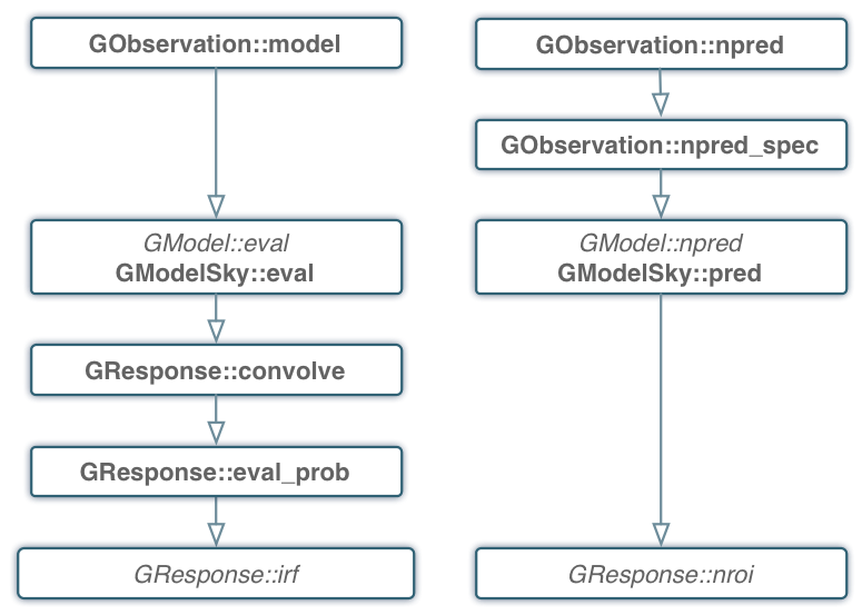
Call tree for model evaluation and IRF convolution

A maximum likelihood analysis of the data generally needs the computation of the predicted number of events within the selection region for each source model. Selection region means here the range of measured quantities that is used for analysis (i.e. range in event position \(p'\), measured energy \(E'\) and time \(t'\)). For a likelihood analysis where the events have been binned in a data cube (i.e. a so-called binned likelihood analysis), the predicted number of events is obtained by summing over all bins of the predicted events in the data cube. For an unbinned likelihood analysis that operates directly on the list of detected events, the predicted number of events is obtained by integrating equation (1) over the selection region:

(3)\[N_{\rm pred} = \int_{\rm GTI} \int_{E_{\rm bounds}} \int_{\rm ROI} P(p', E', t') \, {\rm d}p' \, {\rm d}E' \, {\rm d}t'\]

Here, the event selection region is defined by a Region of Interest (\(\rm ROI\)) that defines the selected range in event positions \(p'\), a set of energy boundaries (\(E_{\rm bounds}\)) that defines the selected energies \(E'\), and Good Time Intervals (\(\rm GTI\)) that the define the selected time intervals. The definition of the Region of Interest is instrument specific and needs to be implemented by a class derived from the abstract GRoi class. Energy boundaries are specified by the GEbounds class, time intervals by the GGti class.

The integration over the region of interest

\[N_{\rm ROI} = \int_{\rm ROI} (p', E', t') \, {\rm d}p'\]

is provided by the GResponse::nroi(GModelSky&, GEnergy&, GTime&, GObservation&) method (see figure above for the call tree).

A final word about deadtime corrections. Deadtime corrections need to be taken into account at the level of the instrument specific response classes. Deadtime corrections can be determined using the GObservation::deadc() method, which provides the time dependent deadtime correction factor.