Model handling¶

Overview¶

The following figure presents an overview over the C++ classes of the model module and their relations.

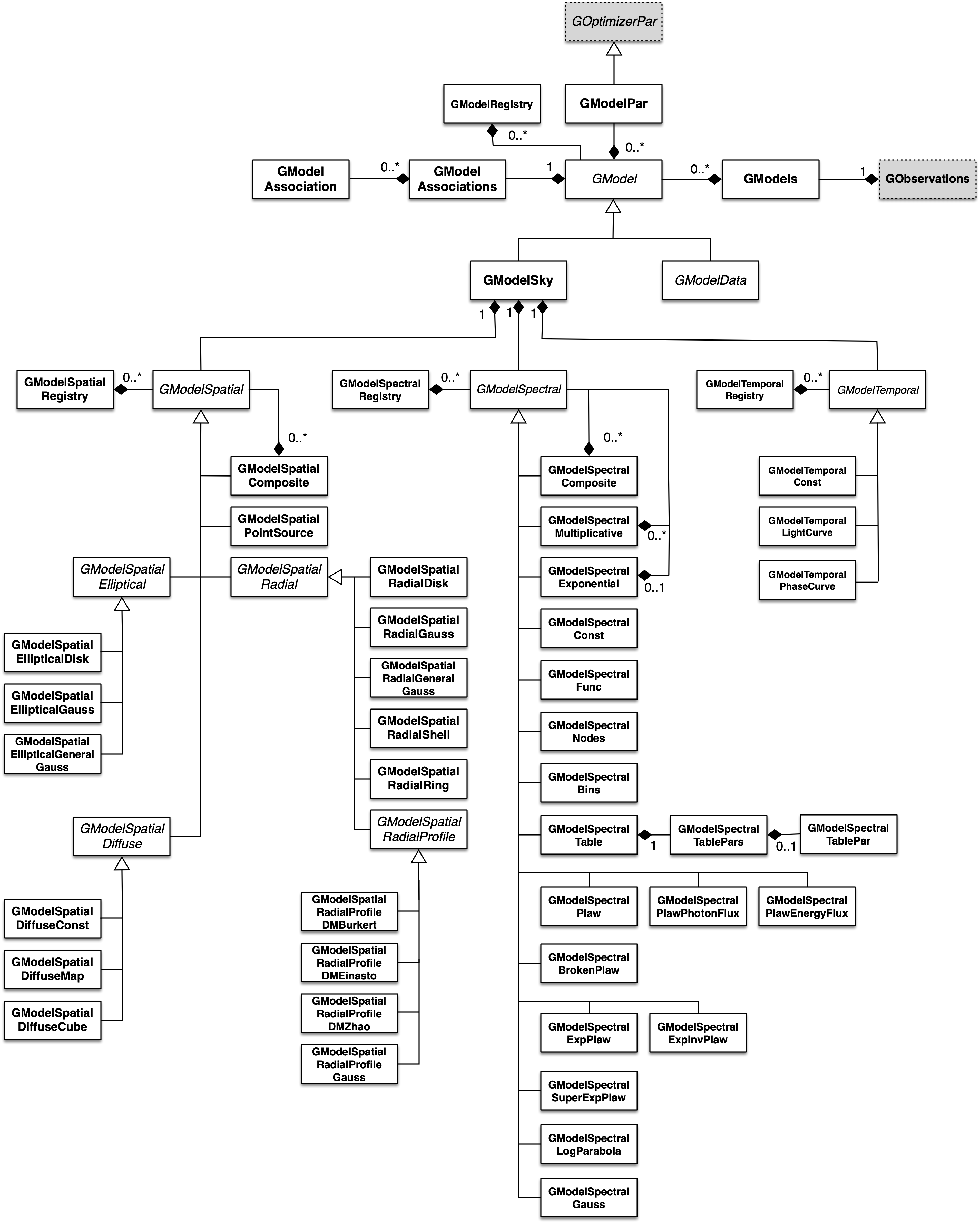
Overview over the model module

The central C++ class of the model module is the abstract base class GModel which defines a model component. Model components are combined using the GModels container C++ class.

Sky models¶

Model factorisation¶

Sky models describe the spatial, spectral and temporal properties of a gamma-ray source using the following factorisation:

\[M(p,E,t) = M_{\rm spatial}(p | E,t) \times M_{\rm spectral}(E | t) \times M_{\rm temporal}(t)\]

(\(M(p,E,t)\) is given in units of \(photons \,\, cm^{-2} s^{-1} MeV^{-1} sr^{-1}\)). The spatial model component \(M_{\rm spatial}(p|E,t)\) is defined by the abstract GModelSpatial class, the spectral model component \(M_{\rm spectral}(E|t)\) is defined by the abstract GModelSpectral class and the temporal component \(M_{\rm temporal}(t)\) is defined by the abstract GModelTemporal class.

The spatial model component describes the energy and time dependent morphology of the source. It satisfies

\[\int_{\Omega} M_{\rm spatial}(p|E,t) \, d\Omega = 1\]

for all \(E\) and \(t\), hence the spatial component does not impact the spatially integrated spectral and temporal properties of the source (the integration is done here over the spatial parameters \(p\) in a spherical coordinate system). The units of the spatial model component are \([M_{\rm spatial}] = {\rm sr}^{-1}\).

The spectral model component describes the spatially integrated time dependent spectral distribution of the source. It satisfies

\[\int_{E} M_{\rm spectral}(E | t) \, dE = \Phi\]

for all \(t\), where \(\Phi\) is the spatially and spectrally integrated total source flux. The spectral component does not impact the temporal properties of the integrated flux \(\Phi\). The units of the spectral model component are \([M_{\rm spectral}] = {\rm cm}^{-2} {\rm s}^{-1} {\rm MeV}^{-1}\).

The temporal model component describes the relative variation of the source flux with respect to the mean value given by the spectral model component. The temporal model component is unit less.

XML model definition format¶

Sky models can be defined using an XML file format that is inspired by the format used for the Large Area Telescope (LAT) aboard NASA’s Fermi satellite. To illustrate the format, the definition of a point source at the position of the Crab nebula with a power spectral shape is shown below. The tags <spatialModel>, <spectrum> and <temporalModel> describe the spatial, spectral and temporal model components defined above. The <temporalModel> tag can be omitted, which will automatically allocate a constant temporal component for the model.

Each source model needs to have a unique name specified by the name attributes. The type attribute specifies the type of the model and needs to be one of PointSource, ExtendedSource, DiffuseSource and CompositeSource. Optional attributes include:

id, specifying an identifier string for a model that can be used to tie the source model to one or several observations;,
ts, specifying the Test Statistic value of the source model component, and
tscalc, specifying whether the Test Statistic value should be computed in a maximum-likelihood computation.

<?xml version="1.0" standalone="no"?>
<source_library title="source library">
  <source name="Crab" type="PointSource">
    <spatialModel type="PointSource">
      <parameter name="RA"  scale="1.0" value="83.6331" min="-360" max="360" free="1"/>
      <parameter name="DEC" scale="1.0" value="22.0145" min="-90"  max="90"  free="1"/>
    </spatialModel>
    <spectrum type="PowerLaw">
      <parameter name="Prefactor"   scale="1e-16" value="5.7"  min="1e-07" max="1000.0" free="1"/>
      <parameter name="Index"       scale="-1"    value="2.48" min="0.0"   max="+5.0"   free="1"/>
      <parameter name="PivotEnergy" scale="1e6"   value="0.3"  min="0.01"  max="1000.0" free="0"/>
    </spectrum>
    <temporalModel type="Constant">
      <parameter name="Normalization" scale="1.0" value="1.0" min="0.1" max="10.0" free="0"/>
    </temporalModel>
  </source>
</source_library>

To accomodate for possible calibration biases for different instruments, instrument specific scaling factors can be specified as part of a model. In the example below, the model will be multiplied by a factor of 1 for LAT and a factor of 0.5 for CTA.

<?xml version="1.0" standalone="no"?>
<source_library title="source library">
  <source name="Crab" type="PointSource">
    ...
    <scaling>
      <instrument name="LAT" scale="1.0" min="0.1" max="10.0" value="1.0" free="0"/>
      <instrument name="CTA" scale="1.0" min="0.1" max="10.0" value="0.5" free="0"/>
    </scaling>
  </source>
</source_library>

Spatial components¶

Point source¶

<source name="Crab" type="PointSource">
  <spatialModel type="PointSource">
    <parameter name="RA"  scale="1.0" value="83.6331" min="-360" max="360" free="1"/>
    <parameter name="DEC" scale="1.0" value="22.0145" min="-90"  max="90"  free="1"/>
  </spatialModel>
  <spectrum type="...">
    ...
  </spectrum>
</source>

An alternative XML format is supported for compatibility with the Fermi/LAT XML format:

<source name="Crab" type="PointSource">
  <spatialModel type="SkyDirFunction">
    <parameter name="RA"  scale="1.0" value="83.6331" min="-360" max="360" free="1"/>
    <parameter name="DEC" scale="1.0" value="22.0145" min="-90"  max="90"  free="1"/>
  </spatialModel>
  <spectrum type="...">
    ...
  </spectrum>
</source>

Radial disk¶

<source name="Crab" type="ExtendedSource">
  <spatialModel type="RadialDisk">
    <parameter name="RA"     scale="1.0" value="83.6331" min="-360" max="360" free="1"/>
    <parameter name="DEC"    scale="1.0" value="22.0145" min="-90"  max="90"  free="1"/>
    <parameter name="Radius" scale="1.0" value="0.20"    min="0.01" max="10"  free="1"/>
  </spatialModel>
  <spectrum type="...">
    ...
  </spectrum>
</source>

Radial Gaussian¶

<source name="Crab" type="ExtendedSource">
  <spatialModel type="RadialGaussian">
    <parameter name="RA"    scale="1.0" value="83.6331" min="-360" max="360" free="1"/>
    <parameter name="DEC"   scale="1.0" value="22.0145" min="-90"  max="90"  free="1"/>
    <parameter name="Sigma" scale="1.0" value="0.20"    min="0.01" max="10"  free="1"/>
  </spatialModel>
  <spectrum type="...">
    ...
  </spectrum>
</source>

Radial shell¶

<source name="Crab" type="ExtendedSource">
  <spatialModel type="RadialShell">
    <parameter name="RA"     scale="1.0" value="83.6331" min="-360" max="360" free="1"/>
    <parameter name="DEC"    scale="1.0" value="22.0145" min="-90"  max="90"  free="1"/>
    <parameter name="Radius" scale="1.0" value="0.30"    min="0.01" max="10"  free="1"/>
    <parameter name="Width"  scale="1.0" value="0.10"    min="0.01" max="10"  free="1"/>
  </spatialModel>
  <spectrum type="...">
    ...
  </spectrum>
</source>

Elliptical disk¶

<source name="Crab" type="ExtendedSource">
  <spatialModel type="EllipticalDisk">
    <parameter name="RA"          scale="1.0" value="83.6331" min="-360"  max="360" free="1"/>
    <parameter name="DEC"         scale="1.0" value="22.0145" min="-90"   max="90"  free="1"/>
    <parameter name="PA"          scale="1.0" value="45.0"    min="-360"  max="360" free="1"/>
    <parameter name="MinorRadius" scale="1.0" value="0.5"     min="0.001" max="10"  free="1"/>
    <parameter name="MajorRadius" scale="1.0" value="2.0"     min="0.001" max="10"  free="1"/>
  </spatialModel>
  <spectrum type="...">
    ...
  </spectrum>
</source>

Elliptical Gaussian¶

<source name="Crab" type="ExtendedSource">
  <spatialModel type="EllipticalGaussian">
    <parameter name="RA"          scale="1.0" value="83.6331" min="-360"  max="360" free="1"/>
    <parameter name="DEC"         scale="1.0" value="22.0145" min="-90"   max="90"  free="1"/>
    <parameter name="PA"          scale="1.0" value="45.0"    min="-360"  max="360" free="1"/>
    <parameter name="MinorRadius" scale="1.0" value="0.5"     min="0.001" max="10"  free="1"/>
    <parameter name="MajorRadius" scale="1.0" value="2.0"     min="0.001" max="10"  free="1"/>
  </spatialModel>
  <spectrum type="...">
    ...
  </spectrum>
</source>

Isotropic source¶

<source name="Crab" type="DiffuseSource">
  <spatialModel type="DiffuseIsotropic">
     <parameter name="Value" scale="1" value="1" min="1"  max="1" free="0"/>
  </spatialModel>
  <spectrum type="...">
    ...
  </spectrum>
</source>

An alternative XML format is supported for compatibility with the Fermi/LAT XML format:

<source name="Crab" type="DiffuseSource">
  <spatialModel type="ConstantValue">
     <parameter name="Value" scale="1" value="1" min="1"  max="1" free="0"/>
  </spatialModel>
  <spectrum type="...">
    ...
  </spectrum>
</source>

Diffuse map¶

<source name="Crab" type="DiffuseSource">
  <spatialModel type="DiffuseMap" file="map.fits">
     <parameter name="Normalization" scale="1" value="1" min="0.001" max="1000.0" free="0"/>
  </spatialModel>
  <spectrum type="...">
    ...
  </spectrum>
</source>

An alternative XML format is supported for compatibility with the Fermi/LAT XML format:

<source name="Crab" type="DiffuseSource">
  <spatialModel type="SpatialMap" file="map.fits">
     <parameter name="Prefactor" scale="1" value="1" min="0.001" max="1000.0" free="0"/>
  </spatialModel>
  <spectrum type="...">
    ...
  </spectrum>
</source>

Diffuse map cube¶

<source name="Crab" type="DiffuseSource">
  <spatialModel type="DiffuseMapCube" file="map_cube.fits">
    <parameter name="Normalization" scale="1" value="1" min="0.001" max="1000.0" free="0"/>
  </spatialModel>
  <spectrum type="...">
    ...
  </spectrum>
</source>

An alternative XML format is supported for compatibility with the Fermi/LAT XML format:

<source name="Crab" type="DiffuseSource">
  <spatialModel type="MapCubeFunction" file="map_cube.fits">
    <parameter name="Value" scale="1" value="1" min="0.001" max="1000.0" free="0"/>
  </spatialModel>
  <spectrum type="...">
    ...
  </spectrum>
</source>

Composite model¶

Spatial model components can be combined into a single model using the GModelSpatialComposite class. The class computes

\[M_{\rm spatial}(p|E,t) = \frac{1}{N} \sum_{i=0}^{N-1} M_{\rm spatial}^{(i)}(p|E,t)\]

where \(M_{\rm spatial}^{(i)}(p|E,t)\) is any spatial model component (including another composite model), and \(N\) is the number of model components that are combined.

An example of an XML file for a composite spatial model is shown below. In this example, a point source is added to a radial Gaussian source to form a composite spatial model. All spatial parameters of the composite model are fitted.

<source name="Crab" type="CompositeSource">
  <spatialModel type="Composite">
    <spatialModel type="PointSource" component="PointSource">
      <parameter name="RA"    scale="1.0" value="83.6331" min="-360" max="360" free="1"/>
      <parameter name="DEC"   scale="1.0" value="22.0145" min="-90"  max="90"  free="1"/>
    </spatialModel>
    <spatialModel type="RadialGaussian">
      <parameter name="RA"    scale="1.0" value="83.6331" min="-360" max="360" free="1"/>
      <parameter name="DEC"   scale="1.0" value="22.0145" min="-90"  max="90"  free="1"/>
      <parameter name="Sigma" scale="1.0" value="0.20"    min="0.01" max="10"  free="1"/>
    </spatialModel>
  </spatialModel>
  <spectrum type="...">
    ...
  </spectrum>
</source>

Spectral components¶

Constant¶

The GModelSpectralConst class implements the constant function

\[\frac{dN}{dE} = N_0\]

where the parameters in the XML definition have the following mappings:

\(N_0\) = Normalization

The XML format for specifying a constant is:

<spectrum type="Constant">
 <parameter name="Normalization" scale="1e-16" value="5.7"  min="1e-07" max="1000.0" free="1"/>
</spectrum>

An alternative XML format is supported for compatibility with the Fermi/LAT XML format:

<spectrum type="ConstantValue">
 <parameter name="Value" scale="1e-16" value="5.7"  min="1e-07" max="1000.0" free="1"/>
</spectrum>

Node function¶

The generalisation of the broken power law is the node function, which is defined by a set of energy and intensity values, the so called nodes, which are connected by power laws.

The XML format for specifying a node function is:

<spectrum type="NodeFunction">
 <node>
   <parameter scale="1.0"   name="Energy"    min="0.1"   max="1.0e20" value="1.0"  free="0"/>
   <parameter scale="1e-07" name="Intensity" min="1e-07" max="1000.0" value="1.0"  free="1"/>
 </node>
 <node>
   <parameter scale="1.0"   name="Energy"    min="0.1"   max="1.0e20" value="10.0" free="0"/>
   <parameter scale="1e-07" name="Intensity" min="1e-07" max="1000.0" value="0.1"  free="1"/>
 </node>
</spectrum>

(in this example there are two nodes; the number of nodes in a node function is arbitrary).

File function¶

A function defined using an input ASCII file with columns of energy and differential flux values. The energy values are assumed to be in units of MeV, the flux values are normally assumed to be in units of \({\rm cm}^{-2} {\rm s}^{-1} {\rm MeV}^{-1}\).

The only parameter of the model is a multiplicative normalization:

\[\frac{dN}{dE} = N_0 \left. \frac{dN}{dE} \right\rvert_{\rm file}\]

where the parameters in the XML definition have the following mappings:

\(N_0\) = Normalization

The XML format for specifying a file function is:

<spectrum type="FileFunction" file="data/filefunction.txt">
 <parameter scale="1.0" name="Normalization" min="0.0" max="1000.0" value="1.0" free="1"/>
</spectrum>

If the file attribute is a relative path, the path is relative to the directory where the XML file resides. Alternatively, an absolute path may be specified. Any environment variable present in the path name will be expanded.

Power law¶

The GModelSpectralPlaw class implements the power law function

\[\frac{dN}{dE} = k_0 \left( \frac{E}{E_0} \right)^{\gamma}\]

where the parameters in the XML definition have the following mappings:

\(k_0\) = Prefactor
\(\gamma\) = Index
\(E_0\) = PivotEnergy

The XML format for specifying a power law is:

<spectrum type="PowerLaw">
 <parameter name="Prefactor"   scale="1e-16" value="5.7"  min="1e-07" max="1000.0" free="1"/>
 <parameter name="Index"       scale="-1"    value="2.48" min="0.0"   max="+5.0"   free="1"/>
 <parameter name="PivotEnergy" scale="1e6"   value="0.3"  min="0.01"  max="1000.0" free="0"/>
</spectrum>

An alternative XML format is supported for compatibility with the Fermi/LAT XML format:

<spectrum type="PowerLaw">
 <parameter name="Prefactor" scale="1e-16" value="5.7"  min="1e-07" max="1000.0" free="1"/>
 <parameter name="Index"     scale="-1"    value="2.48" min="0.0"   max="+5.0"   free="1"/>
 <parameter name="Scale"     scale="1e6"   value="0.3"  min="0.01"  max="1000.0" free="0"/>
</spectrum>

An alternative power law function is defined by the GModelSpectralPlawPhotonFlux class that uses the integral photon flux as parameter rather than the Prefactor:

\[\frac{dN}{dE} = \frac{F_{\rm ph}(\gamma+1)E^{\gamma}} {E_{\rm max}^{\gamma+1} - E_{\rm min}^{\gamma+1}}\]

where the parameters in the XML definition have the following mappings:

\(F_{\rm ph}\) = PhotonFlux
\(\gamma\) = Index
\(E_{\rm min}\) = LowerLimit
\(E_{\rm max}\) = UpperLimit

The XML format for specifying a power law defined by the integral photon flux is:

<spectrum type="PowerLaw">
 <parameter scale="1e-07" name="PhotonFlux" min="1e-07" max="1000.0"    value="1.0"      free="1"/>
 <parameter scale="1.0"   name="Index"      min="-5.0"  max="+5.0"      value="-2.0"     free="1"/>
 <parameter scale="1.0"   name="LowerLimit" min="10.0"  max="1000000.0" value="100.0"    free="0"/>
 <parameter scale="1.0"   name="UpperLimit" min="10.0"  max="1000000.0" value="500000.0" free="0"/>
</spectrum>

An alternative XML format is supported for compatibility with the Fermi/LAT XML format:

<spectrum type="PowerLaw2">
 <parameter scale="1e-07" name="Intergal"   min="1e-07" max="1000.0"    value="1.0"      free="1"/>
 <parameter scale="1.0"   name="Index"      min="-5.0"  max="+5.0"      value="-2.0"     free="1"/>
 <parameter scale="1.0"   name="LowerLimit" min="10.0"  max="1000000.0" value="100.0"    free="0"/>
 <parameter scale="1.0"   name="UpperLimit" min="10.0"  max="1000000.0" value="500000.0" free="0"/>
</spectrum>

Note

The UpperLimit and LowerLimit parameters are always treated as fixed and, as should be apparent from this definition, the flux given by the PhotonFlux parameter is over the range [LowerLimit, UpperLimit]. Use of this model allows the errors on the integrated photon flux to be evaluated directly by likelihood, obviating the need to propagate the errors if one is using the PowerLaw form.

Another alternative power law function is defined by the GModelSpectralPlawEnergyFlux class that uses the integral energy flux as parameter rather than the Prefactor:

\[\frac{dN}{dE} = \frac{F_{\rm E}(\gamma+2)E^{\gamma}} {E_{\rm max}^{\gamma+2} - E_{\rm min}^{\gamma+2}}\]

where the parameters in the XML definition have the following mappings:

\(F_{\rm E}\) = EnergyFlux
\(\gamma\) = Index
\(E_{\rm min}\) = LowerLimit
\(E_{\rm max}\) = UpperLimit

The XML format for specifying a power law defined by the integral energy flux is:

<spectrum type="PowerLaw">
 <parameter scale="1e-07" name="EnergyFlux" min="1e-07" max="1000.0"    value="1.0"      free="1"/>
 <parameter scale="1.0"   name="Index"      min="-5.0"  max="+5.0"      value="-2.0"     free="1"/>
 <parameter scale="1.0"   name="LowerLimit" min="10.0"  max="1000000.0" value="100.0"    free="0"/>
 <parameter scale="1.0"   name="UpperLimit" min="10.0"  max="1000000.0" value="500000.0" free="0"/>
</spectrum>

Note

The UpperLimit and LowerLimit parameters are always treated as fixed and, as should be apparent from this definition, the flux given by the EnergyFlux parameter is over the range [LowerLimit, UpperLimit]. Use of this model allows the errors on the integrated energy flux to be evaluated directly by likelihood, obviating the need to propagate the errors if one is using the PowerLaw form.

Exponentially cut-off power law¶

The GModelSpectralExpPlaw class implements the exponentially cut-off power law function

\[\frac{dN}{dE} = k_0 \left( \frac{E}{E_0} \right)^{\gamma} \exp \left( \frac{-E}{E_{\rm cut}} \right)\]

where the parameters in the XML definition have the following mappings:

\(k_0\) = Prefactor
\(\gamma\) = Index
\(E_0\) = PivotEnergy
\(E_{\rm cut}\) = CutoffEnergy

The XML format for specifying an exponentially cut-off power law is:

<spectrum type="ExponentialCutoffPowerLaw">
 <parameter name="Prefactor"    scale="1e-16" value="5.7"  min="1e-07" max="1000.0" free="1"/>
 <parameter name="Index"        scale="-1"    value="2.48" min="0.0"   max="+5.0"   free="1"/>
 <parameter name="CutoffEnergy" scale="1e6"   value="1.0"  min="0.01"  max="1000.0" free="1"/>
 <parameter name="PivotEnergy"  scale="1e6"   value="0.3"  min="0.01"  max="1000.0" free="0"/>
</spectrum>

An alternative XML format is supported for compatibility with the Fermi/LAT XML format:

<spectrum type="ExpCutoff">
 <parameter name="Prefactor" scale="1e-16" value="5.7"  min="1e-07" max="1000.0" free="1"/>
 <parameter name="Index"     scale="-1"    value="2.48" min="0.0"   max="+5.0"   free="1"/>
 <parameter name="Cutoff"    scale="1e6"   value="1.0"  min="0.01"  max="1000.0" free="1"/>
 <parameter name="Scale"     scale="1e6"   value="0.3"  min="0.01"  max="1000.0" free="0"/>
</spectrum>

An alternative exponentially cut-off power law function is defined by the GModelSpectralExpInvPlaw class which makes use of the inverse of the cut-off energy for function parametrisation:

\[\frac{dN}{dE} = k_0 \left( \frac{E}{E_0} \right)^{\gamma} \exp \left( -\lambda E \right)\]

where the parameters in the XML definition have the following mappings:

\(k_0\) = Prefactor
\(\gamma\) = Index
\(E_0\) = PivotEnergy
\(\lambda\) = InverseCutoffEnergy

The XML format for specifying an exponentially cut-off power law using this alternative parametrisation is:

<spectrum type="ExponentialCutoffPowerLaw">
 <parameter name="Prefactor"           scale="1e-16" value="5.7"  min="1e-07" max="1000.0" free="1"/>
 <parameter name="Index"               scale="-1"    value="2.48" min="0.0"   max="+5.0"   free="1"/>
 <parameter name="InverseCutoffEnergy" scale="1e-6"  value="1.0"  min="0.0"   max="100.0"  free="1"/>
 <parameter name="PivotEnergy"         scale="1e6"   value="0.3"  min="0.01"  max="1000.0" free="0"/>
</spectrum>

Super exponentially cut-off power law¶

The GModelSpectralSuperExpPlaw class implements the super exponentially cut-off power law function

\[\frac{dN}{dE} = k_0 \left( \frac{E}{E_0} \right)^{\gamma} \exp \left( -\left( \frac{E}{E_{\rm cut}} \right)^{\alpha} \right)\]

where the parameters in the XML definition have the following mappings:

\(k_0\) = Prefactor
\(\gamma\) = Index1
\(\alpha\) = Index2
\(E_0\) = PivotEnergy
\(E_{\rm cut}\) = CutoffEnergy

<spectrum type="SuperExponentialCutoffPowerLaw">
 <parameter name="Prefactor"    scale="1e-16" value="1.0" min="1e-07" max="1000.0" free="1"/>
 <parameter name="Index1"       scale="-1"    value="2.0" min="0.0"   max="+5.0"   free="1"/>
 <parameter name="CutoffEnergy" scale="1e6"   value="1.0" min="0.01"  max="1000.0" free="1"/>
 <parameter name="Index2"       scale="1.0"   value="1.5" min="0.1"   max="5.0"    free="1"/>
 <parameter name="PivotEnergy"  scale="1e6"   value="1.0" min="0.01"  max="1000.0" free="0"/>
</spectrum>

An alternative XML format is supported for compatibility with the Fermi/LAT XML format:

<spectrum type="PLSuperExpCutoff">
 <parameter name="Prefactor"   scale="1e-16" value="1.0" min="1e-07" max="1000.0" free="1"/>
 <parameter name="Index1"      scale="-1"    value="2.0" min="0.0"   max="+5.0"   free="1"/>
 <parameter name="Cutoff"      scale="1e6"   value="1.0" min="0.01"  max="1000.0" free="1"/>
 <parameter name="Index2"      scale="1.0"   value="1.5" min="0.1"   max="5.0"    free="1"/>
 <parameter name="Scale"       scale="1e6"   value="1.0" min="0.01"  max="1000.0" free="0"/>
</spectrum>

Broken power law¶

The GModelSpectralBrokenPlaw class implements the broken power law function

\[\begin{split}\frac{dN}{dE} = k_0 \times \left \{ \begin{eqnarray} \left( \frac{E}{E_b} \right)^{\gamma_1} & {\rm if\,\,} E < E_b \\ \left( \frac{E}{E_b} \right)^{\gamma_2} & {\rm otherwise} \end{eqnarray} \right .\end{split}\]

where the parameters in the XML definition have the following mappings:

\(k_0\) = Prefactor
\(\gamma_1\) = Index1
\(\gamma_2\) = Index2
\(E_b\) = BreakEnergy

The XML format for specifying a broken power law is:

<spectrum type="BrokenPowerLaw">
 <parameter name="Prefactor"   scale="1e-16" value="5.7"  min="1e-07" max="1000.0" free="1"/>
 <parameter name="Index1"      scale="-1"    value="2.48" min="0.0"   max="+5.0"   free="1"/>
 <parameter name="BreakEnergy" scale="1e6"   value="0.3"  min="0.01"  max="1000.0" free="1"/>
 <parameter name="Index2"      scale="-1"    value="2.70" min="0.01"  max="1000.0" free="1"/>
</spectrum>

An alternative XML format is supported for compatibility with the Fermi/LAT XML format:

<spectrum type="BrokenPowerLaw">
 <parameter name="Prefactor"  scale="1e-16" value="5.7"  min="1e-07" max="1000.0" free="1"/>
 <parameter name="Index1"     scale="-1"    value="2.48" min="0.0"   max="+5.0"   free="1"/>
 <parameter name="BreakValue" scale="1e6"   value="0.3"  min="0.01"  max="1000.0" free="1"/>
 <parameter name="Index2"     scale="-1"    value="2.70" min="0.01"  max="1000.0" free="1"/>
</spectrum>

Smoothly broken power law¶

The GModelSpectralSmoothBrokenPlaw class implements the smoothly broken power law function

\[\frac{dN}{dE} = k_0 \left( \frac{E}{E_0} \right)^{\gamma_1} \left[ 1 + \left( \frac{E}{E_b} \right)^{\frac{\gamma_1 - \gamma_2}{\beta}} \right]^{-\beta}\]

where the parameters in the XML definition have the following mappings:

\(k_0\) = Prefactor
\(\gamma_1\) = Index1
\(E_0\) = PivotEnergy
\(\gamma_2\) = Index2
\(E_b\) = BreakEnergy
\(\beta\) = BreakSmoothness

The XML format for specifying a smoothly broken power law is:

<spectrum type="SmoothBrokenPowerLaw">
  <parameter name="Prefactor"       scale="1e-16" value="5.7"  min="1e-07" max="1000.0" free="1"/>
  <parameter name="Index1"          scale="-1"    value="2.48" min="0.0"   max="+5.0"   free="1"/>
  <parameter name="PivotEnergy"     scale="1e6"   value="1.0"  min="0.01"  max="1000.0" free="0"/>
  <parameter name="Index2"          scale="-1"    value="2.70" min="0.01"  max="+5.0"   free="1"/>
  <parameter name="BreakEnergy"     scale="1e6"   value="0.3"  min="0.01"  max="1000.0" free="1"/>
  <parameter name="BreakSmoothness" scale="1.0"   value="0.2"  min="0.01"  max="10.0"   free="0"/>
</spectrum>

An alternative XML format is supported for compatibility with the Fermi/LAT XML format:

<spectrum type="SmoothBrokenPowerLaw">
  <parameter name="Prefactor"   scale="1e-16" value="5.7"  min="1e-07" max="1000.0" free="1"/>
  <parameter name="Index1"      scale="-1"    value="2.48" min="0.0"   max="+5.0"   free="1"/>
  <parameter name="Scale"       scale="1e6"   value="1.0"  min="0.01"  max="1000.0" free="0"/>
  <parameter name="Index2"      scale="-1"    value="2.70" min="0.01"  max="+5.0"   free="1"/>
  <parameter name="BreakValue"  scale="1e6"   value="0.3"  min="0.01"  max="1000.0" free="1"/>
  <parameter name="Beta"        scale="1.0"   value="0.2"  min="0.01"  max="10.0"   free="0"/>
</spectrum>

Gaussian¶

The GModelSpectralGauss class implements the gaussian function

\[\frac{dN}{dE} = \frac{N_0}{\sqrt{2\pi}\sigma} \exp \left( \frac{-(E-\bar{E})^2}{2 \sigma^2} \right)\]

where the parameters in the XML definition have the following mappings:

\(N_0\) = Normalization
\(\bar{E}\) = Mean
\(\sigma\) = Sigma

The XML format for specifying a Gaussian is:

<spectrum type="Gaussian">
 <parameter name="Normalization" scale="1e-10" value="1.0"  min="1e-07" max="1000.0" free="1"/>
 <parameter name="Mean"          scale="1e6"   value="5.0"  min="0.01"  max="100.0"  free="1"/>
 <parameter name="Sigma"         scale="1e6"   value="1.0"  min="0.01"  max="100.0"  free="1"/>
</spectrum>

Log parabola¶

The GModelSpectralLogParabola class implements the log parabola function

\[\frac{dN}{dE} = k_0 \left( \frac{E}{E_0} \right)^{\gamma+\eta \ln(E/E_0)}\]

where the parameters in the XML definition have the following mappings:

\(k_0\) = Prefactor
\(\gamma\) = Index
\(\eta\) = Curvature
\(E_0\) = PivotEnergy

The XML format for specifying a log parabola spectrum is:

<spectrum type="LogParabola">
 <parameter name="Prefactor"   scale="1e-17" value="5.878"   min="1e-07" max="1000.0" free="1"/>
 <parameter name="Index"       scale="-1"    value="2.32473" min="0.0"   max="+5.0"   free="1"/>
 <parameter name="Curvature"   scale="-1"    value="0.074"   min="-5.0"  max="+5.0"   free="1"/>
 <parameter name="PivotEnergy" scale="1e6"   value="1.0"     min="0.01"  max="1000.0" free="0"/>
</spectrum>

An alternative XML format is supported for compatibility with the Fermi/LAT XML format:

<spectrum type="LogParabola">
 <parameter name="norm"  scale="1e-17" value="5.878"   min="1e-07" max="1000.0" free="1"/>
 <parameter name="alpha" scale="1"     value="2.32473" min="0.0"   max="+5.0"   free="1"/>
 <parameter name="beta"  scale="1"     value="0.074"   min="-5.0"  max="+5.0"   free="1"/>
 <parameter name="Eb"    scale="1e6"   value="1.0"     min="0.01"  max="1000.0" free="0"/>
</spectrum>

where

alpha = -Index
beta = -Curvature

Composite model¶

Spectral model components can be combined into a single model using the GModelSpectralComposite class. The class computes

\[M_{\rm spectral}(E | t) = \sum_{i=0}^{N-1} M_{\rm spectral}^{(i)}(E | t)\]

where \(M_{\rm spectral}^{(i)}(E | t)\) is any spectral model component (including another composite model), and \(N\) is the number of model components that are combined.

The XML format for specifying a composite spectral model is:

<spectrum type="Composite">
  <spectrum type="PowerLaw" component="SoftComponent">
    <parameter name="Prefactor"   scale="1e-17" value="3"  min="1e-07" max="1000.0" free="1"/>
    <parameter name="Index"       scale="-1"    value="3.5" min="0.0"   max="+5.0"   free="1"/>
    <parameter name="PivotEnergy" scale="1e6"   value="1"  min="0.01"  max="1000.0" free="0"/>
  </spectrum>
  <spectrum type="PowerLaw" component="HardComponent">
    <parameter name="Prefactor"   scale="1e-17" value="5"  min="1e-07" max="1000.0" free="1"/>
    <parameter name="Index"       scale="-1"    value="2.0" min="0.0"   max="+5.0"   free="1"/>
    <parameter name="PivotEnergy" scale="1e6"   value="1"  min="0.01"  max="1000.0" free="0"/>
  </spectrum>
</spectrum>

Multiplicative model¶

Another composite spectral model is the multiplicative spectral model that is implemented by the GModelSpectralMultiplicative class. The class computes

\[M_{\rm spectral}(E | t) = \prod_{i=0}^{N-1} M_{\rm spectral}^{(i)}(E | t)\]

where \(M_{\rm spectral}^{(i)}(E | t)\) is any spectral model component (including another composite or multiplicative model), and \(N\) is the number of model components that are multiplied. This model can for example be used to model any kind of gamma-ray absorption.

The XML format for specifying a multiplicative spectral model is:

<spectrum type="Multiplicative">
  <spectrum type="PowerLaw" component="PowerLawComponent">
    <parameter name="Prefactor"   scale="1e-17" value="1.0"  min="1e-07" max="1000.0" free="1"/>
    <parameter name="Index"       scale="-1"    value="2.48" min="0.0"   max="+5.0"   free="1"/>
    <parameter name="PivotEnergy" scale="1e6"   value="1.0"  min="0.01"  max="1000.0" free="0"/>
  </spectrum>
  <spectrum type="ExponentialCutoffPowerLaw" component="CutoffComponent">
    <parameter name="Prefactor"    scale="1.0" value="1.0" min="1e-07" max="1000.0" free="0"/>
    <parameter name="Index"        scale="1.0" value="0.0" min="-2.0"  max="+2.0"   free="0"/>
    <parameter name="CutoffEnergy" scale="1e6" value="1.0" min="0.01"  max="1000.0" free="1"/>
    <parameter name="PivotEnergy"  scale="1e6" value="1.0" min="0.01"  max="1000.0" free="0"/>
  </spectrum>
</spectrum>

Temporal components¶

Constant¶

The GModelTemporalConst class implements a temporal model that is constant in time and defined by

\[M_{\rm temporal}(t) = N_0\]

where the parameter in the XML definition has the following mapping:

\(N_0\) = Normalization

The XML format for specifying a constant temporal model is:

<temporal type="Constant">
  <parameter name="Normalization" scale="1.0" value="1.0" min="0.1" max="10.0" free="0"/>
</temporal>

Light Curve¶

The GModelTemporalLightCurve class implements a temporal model that defines an arbitrary light curve, defined by a function in a FITS file.

The only parameter of the model is a multiplicative normalization:

\[M_{\rm temporal}(t) = N_0 r(t)\]

where the parameter in the XML definition has the following mapping:

\(N_0\) = Normalization

The XML format for specifying a light curve is:

<temporal type="LightCurve" file="model_temporal_lightcurve.fits">
  <parameter name="Normalization" scale="1" value="1.0" min="0.0" max="1000.0" free="0"/>
</temporal>

If the file attribute is a relative path, the path is relative to the directory where the XML file resides. Alternatively, an absolute path may be specified. Any environment variable present in the path name will be expanded.

The structure of the light curve FITS file is shown in the figure below. The light curve is defined in the first extension of the FITS file and consists of a binary table with the columns TIME and NORM. Times in the TIME columns are given in seconds and are counted with respect to a time reference that is defined in the header of the binary table. Times need to be specified in ascending order. The values in the NORM column specify \(r(t)\) at times \(t\), and should be comprised between 0 and 1.

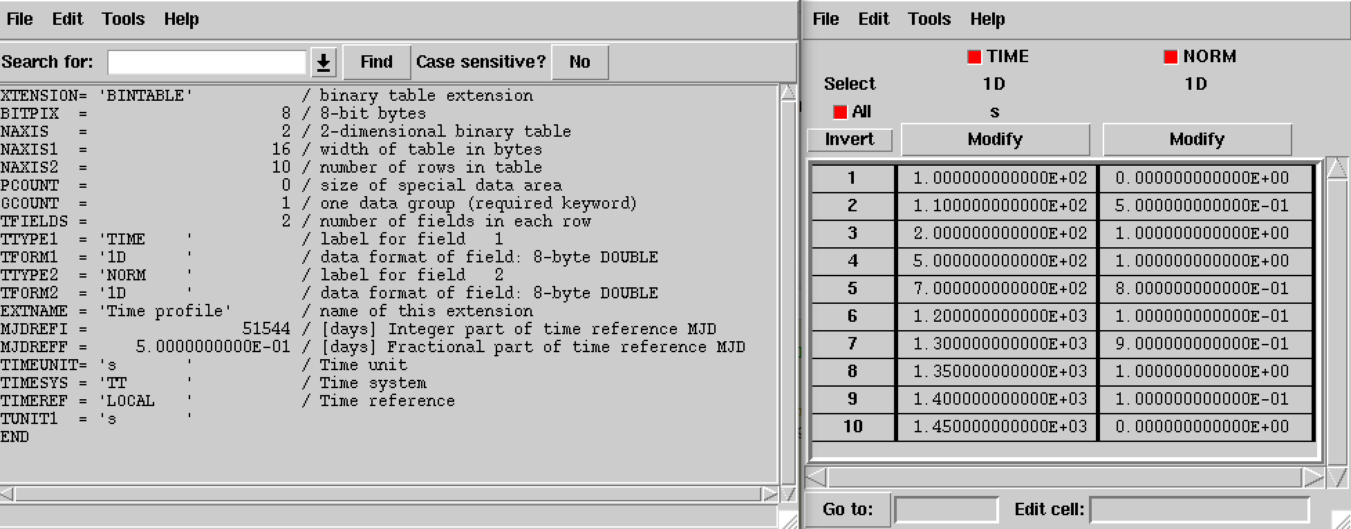
Structure of light curve FITS file

Phase Curve¶

The GModelTemporalPhaseCurve class implements a temporal model that defines a temporal variation based on an arbitrary phase \(\Phi(t)\) that is computed using

\[\Phi(t) = \Phi_0 + f(t-t_0) + \frac{1}{2}\dot{f} (t-t_0)^2 + \frac{1}{6}\ddot{f} (t-t_0)^3\]

where

\(t_0\) is a reference time,
\(\Phi_0\) is the phase at the reference time,
\(f\) is the variation frequency at the reference time,
\(\dot{f}\) is the first derivative of the variation frequency at the reference time, and
\(\ddot{f}\) is the second derivative of the variation frequency at the reference time.

The temporal variation is computed using

\[M_{\rm temporal}(t) = N_0 r(\Phi(t))\]

The parameters in the XML definition have the following mappings:

\(N_0\) = Normalization
\(t_0\) = MJD
\(\Phi_0\) = Phase
\(f\) = F0
\(\dot{f}\) = F1
\(\ddot{f}\) = F2

The XML format for specifying a phase curve is:

<temporal type="PhaseCurve" file="model_temporal_phasecurve.fits">
  <parameter name="Normalization" scale="1" value="1.0"     min="0.0" max="1000.0"   free="0"/>
  <parameter name="MJD"           scale="1" value="51544.5" min="0.0" max="100000.0" free="0"/>
  <parameter name="Phase"         scale="1" value="0.0"     min="0.0" max="1.0"      free="0"/>
  <parameter name="F0"            scale="1" value="1.0"     min="0.0" max="1000.0"   free="0"/>
  <parameter name="F1"            scale="1" value="0.1"     min="0.0" max="1000.0"   free="0"/>
  <parameter name="F2"            scale="1" value="0.01"    min="0.0" max="1000.0"   free="0"/>
</temporal>

If the file attribute is a relative path, the path is relative to the directory where the XML file resides. Alternatively, an absolute path may be specified. Any environment variable present in the path name will be expanded.

The structure of the phase curve FITS file is shown in the figure below. The phase curve is defined in the first extension of the FITS file and consists of a binary table with the columns PHASE and NORM. Phase values in the PHASE column need to be comprised between 0 and 1 and need to be given in ascending order. The values in the NORM column specify \(r(\Phi(t))\) at phases \(\Phi(t)\), and should be comprised between 0 and 1.

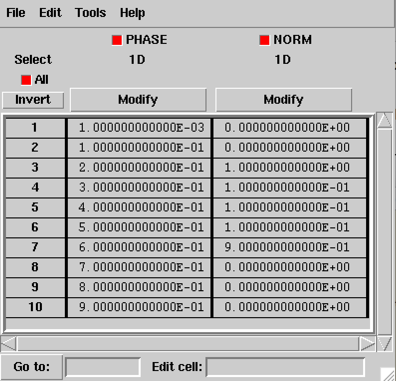
Structure of phase curve FITS file

By default, the NORM values are recomputed internally so that the phase-averaged normalisation is one. In that case, the spectral component corresponds to the phase-averaged spectrum. If the internal normalisation should be disabled the normalize="0" attribute needs to be added to the temporal tag, i.e.

<temporal type="PhaseCurve" file="model_temporal_phasecurve.fits" normalize="0">

In that case the NORM values are directly multiplied with the spectral component.

Background models¶

Background models differ from sky models in that those models are not convolved with the instrument response function, and directly provide the number of predicted background counts as function of measured event properties. Background models need to be implemented in the instrument specific models. All background models derive from the abstract GModelData base class.

Table Of Contents

Previous topic

Next topic

Model handling¶

Overview¶

Sky models¶

Model factorisation¶

XML model definition format¶

Spatial components¶

Point source¶

Radial disk¶

Radial Gaussian¶

Radial shell¶

Elliptical disk¶

Elliptical Gaussian¶

Isotropic source¶

Diffuse map¶

Diffuse map cube¶

Composite model¶

Spectral components¶

Constant¶

Node function¶

File function¶

Power law¶

Exponentially cut-off power law¶

Super exponentially cut-off power law¶

Broken power law¶

Smoothly broken power law¶

Gaussian¶

Log parabola¶

Composite model¶

Multiplicative model¶

Temporal components¶

Constant¶

Light Curve¶

Phase Curve¶

Background models¶