The CTA specific instrument response is described by the GCTAResponseIrf class (see Handling the instrument response for a general description of response handling in GammaLib). The CTA response is factorised into the effective area \(A_{\rm eff}(d, p, E, t)\) (units \(cm^2\)), the point spread function \(PSF(p' | d, p, E, t)\), and the energy dispersion \(E_{\rm disp}(E' | d, p, E, t)\) following:
Three different formats are implemented to specify the response information for CTA: Response Tables, Xspec response files, and Performance tables.
The CTA response table class GCTAResponseTable provides a generic handle for multi-dimensional response information. It is based on the response format used for storing response information for the Fermi/LAT telescope. In this format, all information is stored in a single row of a FITS binary table. Each element of the row contains a vector column, that describes the axes of the multi-dimensional response cube and the response information. Note that this class may in the future be promoted to the GammaLib core, as a similar class has been implemented in the Fermi/LAT interface.
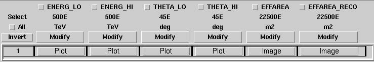
As an example for the format of a response table, the effective area component is shown below. Response information is stored in a n-dimensional cube, and each axis of this cube is described by the lower and upper edges of the axis bins. In this example the effective area is stored as a 2D matrix with the first axis being energy and the second axis being offaxis angle. Effective area information is stored for true (EFFAREA) and reconstructed (EFFAREA_RECO) energy. Vector columns are used to store all information.
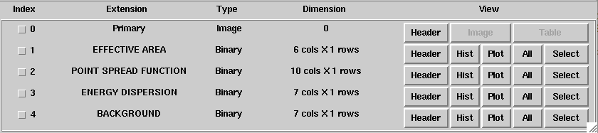
All components of the response ar stored in a single FITS file, and each component of the response factorisation is stored in a binary table of that FITS file. In addition, the response files contain an additional table that describes the background rate as function of energy and position in the field of view. An example of a CTA response file is shown below:
For the first CTA Consortium Data Challenge (1DC) the response information was provided in a format that was inspired from the one use for Xspec. Effective area information after applying a theta cut was given by so called ancilliary response files (ARF files). The energy dispersion was provided as a Redistribution Matrix File (RMF files). There is no Point Spread Function information defined for Xspec, and for the sake of the 1DC, a simple one-dimensional vector had been implemented.
GammaLib still supports handling of the 1DC files, but there are no plans to use this format in the future.
Performance tables specify the CTA on-axis performance as function of energy and have been provided by the Monte Carlo group of the CTA Consortium for a variety of configurations. Performance tables are plain ASCII files. Below an example of a CTA performance table:
log(E)     Area     r68     r80  ERes. BG Rate    Diff Sens
-1.7      261.6  0.3621  0.4908 0.5134 0.0189924  6.88237e-11
-1.5     5458.2  0.2712  0.3685 0.4129 0.1009715  1.72717e-11
-1.3    15590.0  0.1662  0.2103 0.2721 0.0575623  6.16963e-12
-1.1    26554.1  0.1253  0.1567 0.2611 0.0213008  2.89932e-12
-0.9    52100.5  0.1048  0.1305 0.1987 0.0088729  1.39764e-12
-0.7    66132.1  0.0827  0.1024 0.1698 0.0010976  6.03531e-13
-0.5   108656.8  0.0703  0.0867 0.1506 0.0004843  3.98147e-13
-0.3   129833.0  0.0585  0.0722 0.1338 0.0001575  3.23090e-13
-0.1   284604.3  0.0531  0.0656 0.1008 0.0001367  2.20178e-13
 0.1   263175.3  0.0410  0.0506 0.0831 0.0000210  1.87452e-13
 0.3   778048.6  0.0470  0.0591 0.0842 0.0000692  1.53976e-13
 0.5   929818.8  0.0391  0.0492 0.0650 0.0000146  1.18947e-13
 0.7  1078450.0  0.0335  0.0415 0.0541 0.0000116  1.51927e-13
 0.9  1448579.1  0.0317  0.0397 0.0516 0.0000047  1.42439e-13
 1.1  1899905.0  0.0290  0.0372 0.0501 0.0000081  1.96670e-13
 1.3  2476403.8  0.0285  0.0367 0.0538 0.0000059  2.20695e-13
 1.5  2832570.6  0.0284  0.0372 0.0636 0.0000073  3.22523e-13
 1.7  3534065.3  0.0290  0.0386 0.0731 0.0000135  4.84153e-13
 1.9  3250103.4  0.0238  0.0308 0.0729 0.0000044  6.26265e-13
 2.1  3916071.6  0.0260  0.0354 0.0908 0.0000023  7.69921e-13
 ---------------------------------------------
 1) log(E) = log10(E/TeV) - bin centre
 2) Eff Area - in square metres after background cut (no theta cut)
 3) Ang. Res - 68% containment radius of gamma-ray PSF post cuts - in degrees
 4) Ang. Res - 80% containment radius of gamma-ray PSF post cuts - in degrees
 5) Fractional Energy Resolution (rms)
 6) BG Rate  - inside point-source selection region - post call cuts - in Hz
 7) Diff Sens - differential sensitivity for this bin expressed as E^2 dN/dE
    - in erg cm^-2 s^-1 - for a 50 hours exposure - 5 sigma significance including
    systematics and statistics and at least 10 photons.
The \(A_{\rm eff}(d, p, E, t)\) term is described by the abstract GCTAAeff base class. The effective area is determined using the:
double GCTAAeff::operator()(const double& logE,
                            const double& theta = 0.0,
                            const double& phi = 0.0,
                            const double& zenith = 0.0,
                            const double& azimuth = 0.0,
                            const bool&   etrue = true) const;
operator, where logE is the base 10 logarithm of the photon energy. If etrue is true, logE is the true photon energy; otherwise, logE is the measured photon energy. theta and phi are the offset and azimuth angle of the incident photon with respect to the camera pointing, zenith and azimuth are the zenith and azimuth angle of the camera pointing.
The effective area response is implemented by one of the classes GCTAAeffPerfTable, GCTAAeffArf and GCTAAeff2D that implement the different response formats that are currently used in the CTA project. Dependent on the specified response file, the method GCTAResponseIrf::load_aeff() allocates the appropriate response class. GCTAAeff2D is allocated if the response file is a FITS file containing an extension named EFFECTIVE AREA; GCTAAeffArf is allocated if an extension named SPECRESP is found; otherwise, GCTAAeffPerfTable is allocated.
GCTAAeff2D reads the full effective area as function of energies and off-axis angle from a FITS table. The FITS table is expected to be in the Response tables format. From this two-dimensional table, the effective area values are determine by bi-linear interpolation in the base 10 logarithm of photon energy and the offset angle.
GCTAAeffArf extracts the effective area information from a XSPEC compatible ancilliary response file (ARF). The ARF contains the effective area for a specific angular (or theta) cut. It should be noted that the GCTAAeffArf class has been introduced as a work around for digesting the ARF response provided for the 1st CTA Data Challenge (1DC). It is not intended to use this class any longer in the future.
To recover the full effective detection area, the value of the theta cut as well as the form of the point spread function needs to be known. When an ARF file is loaded using the GCTAAeffArf::load() method, the ARF values are read and stored as they are encountered in the ARF file. To recover the full effective detection area the theta cut value has to be specified using the GCTAAeffArf::thetacut() method, and the GCTAAeffArf::remove_thetacut() method needs to be called to rescale the ARF values. Note that GCTAAeffArf::remove_thetacut() shall only be called once after reading the ARF, as every call of the method will modify the effective area values by multiplying it with a scaling factor. The scaling factor required to recover the full effective area will be obtained by integrating the area under the point spread function out to the specified theta cut value. This provides the fraction of all events that should fall within the theta cut. The applied scaling factor is the inverse of this fraction:
An alternative way of selecting the events is to adopt an energy dependent theta cut so that the selection always contains a fixed fraction of the events. This type of cut can be accomodated by specifying a scaling factor using the GCTAAeffArf::scale() method prior to loading the ARF data. For example, if the containment fraction was fixed to 80%, a scaling of 1.25 should be applied to recover the full effective detection area. When response information is specified by an XML file (see Describing CTA observations using XML), the thetacut and scale parameters can be defined using optional attributes to the EffectiveArea parameter.
The ARF format does not provide any information on the off-axis dependence of the response, as the ARF values are supplied for a specific source position, and hence for a specific off-axis angle with respect to the camera centre. By default, the same effective area values are thus applied to all off-axis angles \(\theta\). An off-axis dependence may however be introduced by supplying a positive value for the \(\sigma\) parameter using the GCTAAeffArf::sigma() method, or by adding the sigma attribute to the EffectiveArea parameter in the XML file. In that case, equation (2) is used for the off-axis dependence, with the supplied ARF values being taken as the on-axis values.
GCTAAeffPerfTable reads the effective area information from an ASCII file that has been defined by the CTA Monte Carlo workpackage (see Performance table). This file provides the full effective detection area in units of \(m^2\) after the background cut as function of the base 10 logarithm of the true photon energy. No theta cut is applied. For a given energy, the effective area is computed by interpolating the performance table in the base 10 logarithm of energy. Effective areas will always be non-negative. As the response table provides only the on-axis effective area, off-axis effective areas are estimated assuming that the radial distribution follows a Gaussian distribution in offset angle squared:
where \(\sigma\) characterises the size of the field of view. The \(\sigma\) parameter is set and retrieved using the GCTAAeffPerfTable::sigma() methods. When response information is specified by an XML file (see Describing CTA observations using XML), the \(\sigma\) parameter can be set using the optional sigma attribute. If the \(\sigma\) parameter is not explicitly set, \(\sigma=3 \, {\rm deg}^2\) is assumed as default.
The \(PSF(p' | d, p, E, t)\) term is described by the abstract GCTAPsf base class. The point spread function is determined using the:
double GCTAPsf::operator()(const double& delta,
                           const double& logE,
                           const double& theta = 0.0,
                           const double& phi = 0.0,
                           const double& zenith = 0.0,
                           const double& azimuth = 0.0,
                           const bool&   etrue = true) const;
operator, where delta is the angle between true and measured photon arrival direction and logE is the base 10 logarithm of the photon energy. If etrue is true, logE is the true photon energy; otherwise, logE is the measured photon energy. theta and phi are the offset and azimuth angle of the incident photon with respect to the camera pointing, zenith and azimuth are the zenith and azimuth angle of the camera pointing.
The \(E_{\rm disp}(E' | d, p, E, t)\) term is described by the abstract GCTAEdisp base class. The energy dispersion is determined using the:
double GCTAEdisp::operator()(const double& logEobs,
                             const double& logEsrc,
                             const double& theta = 0.0,
                             const double& phi = 0.0,
                             const double& zenith = 0.0,
                             const double& azimuth = 0.0) const;
operator, where logEobs is the base 10 logarithm of the measured energy, logEsrc is the base 10 logarithm of the true energy, theta and phi are the offset and azimuth angle of the incident photon with respect to the camera pointing, and zenith and azimuth are the zenith and azimuth angle of the camera pointing.
The background is described by the abstract GCTABackground base class. The background is determined using the:
double GCTABackground::operator()(const double& logE,
                                  const double& detx,
                                  const double& dety) const;
operator, where logE is the base 10 logarithm of the measured energy, and detx and dety are the measured arrival directions in the nominal camera system.