The following figure presents an overview over the C++ classes of the obs module and their relations.
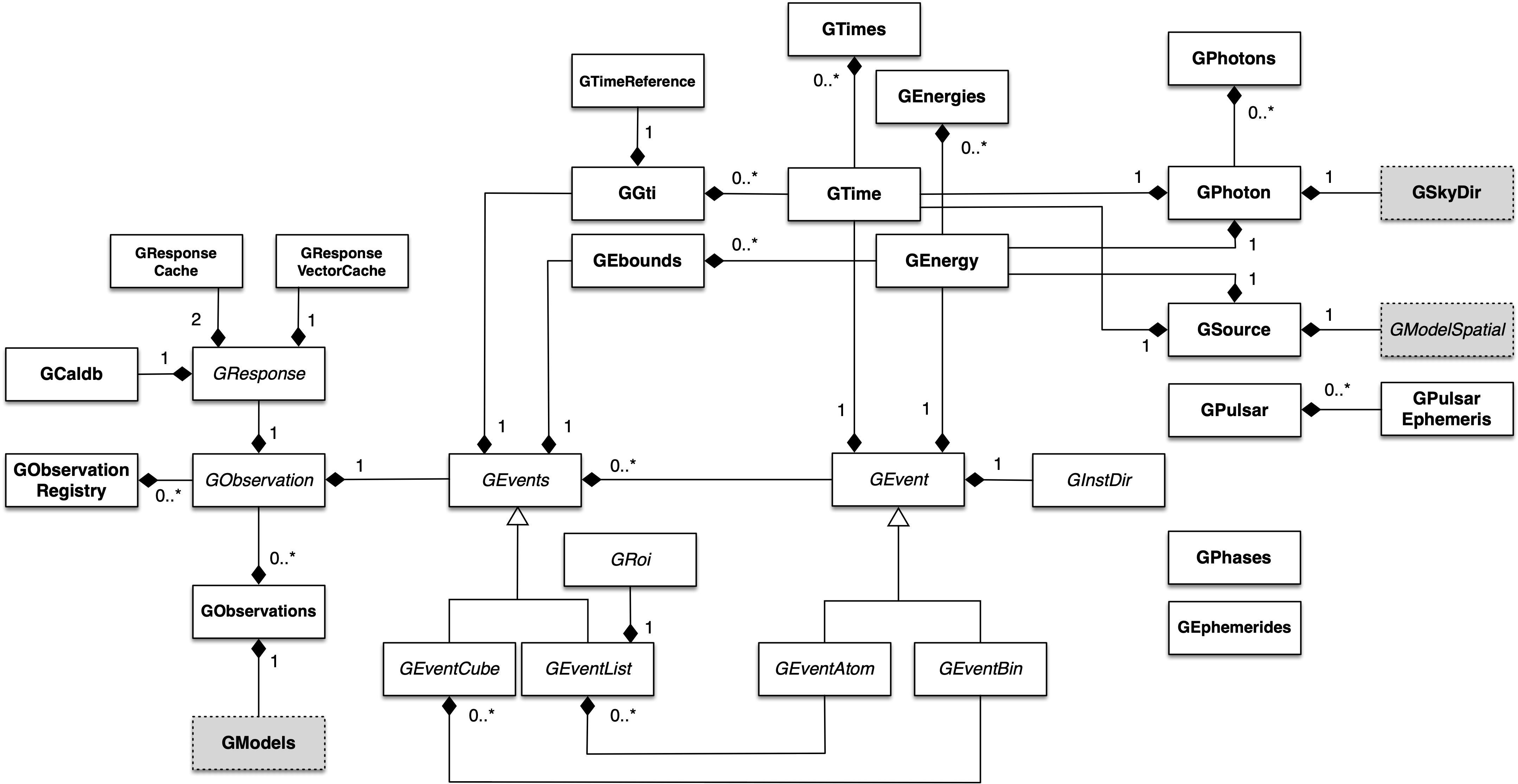
Overview over the obs module
The central C++ class of the obs module is the abstract base class GObservation which defines the instrument-independent interface for a gamma-ray observation. A gamma-ray observation is defined for a single specific instrument, and describes a time period during which the instrument is in a given stable configuration that can be characterized by a single specific response function. Each gamma-ray observation is composed of events and a response function.
Observations are collected in the C++ container class GObservations which is composed of a list of GObservation elements (the list is of arbitrary length; an empty list is a valid state of the GObservations class). The observation container is furthermore composed of a GModels model container class that holds a list of models used to describe the event distributions of the observations (see Model handling). The GObservations class presents the central element of all scientific data analyses, as it combines all data and all models in a single entity.
Instrument specific implementations of GObservation objects are registered in the C++ registry class GObservationRegistry which statically collects one instance of each instrument-specific observation class that is available in GammaLib (see Registry classes for a general description of registry classes).
The instrument response for a given observation is defined by the abstract base class GResponse. This class is composed of the C++ class GCaldb which implements the calibration data base that is required to compute the response function for a given instrument and observation. GCaldb supports the HEASARC CALDB format (http://heasarc.nasa.gov/docs/heasarc/caldb/), but is sufficiently general to support also other formats (see Setting up and using a calibration database to learn how to setup and to use a calibration database).
The events for a given observation are defined by the abstract base class GEvents. This class is composed of the C++ classes GGti and GEbounds. GGti implements so called Good Time Intervals, which defines the time period(s) during which the data were taken (see Times in GammaLib). GEbounds implements so called Energy Boundaries, which define the energy intervals that are covered by the data (see Energies in GammaLib).
GEvents is also a container for the individual events, implemented by the abstract GEvent base class. GammaLib distinguishes two types of events: event atoms, which are individual events, and event bins, which are collections of events with similar properties. Event atoms are implemented by the abstract base class GEventAtom, while event bins are implemented by the abstract base class GEventBin. Both classes derive from the abstract GEvent base class.
Each event type has it’s own container class, which derives from the abstract GEvents base class. Event atoms are collected by the abstract GEventList base class, while event bins are collected by the abstract GEventCube base class. The GEventList class contains an instance of the abstract GRoi base class.
Observations can be described in GammaLib using an ASCII file in XML format. The general format of this file is:
<observation_list title="observation library">
    <observation name="..." id="..." instrument="...">
      ...
    </observation>
    <observation name="..." id="..." instrument="...">
      ...
    </observation>
    ...
</observation_list>
where each <observation> tag describes one observation. Each observation has a name attribute, an id (identifier) attribute and an instrument attribute. The latter decides which instrument specific class will be allocated upon reading the XML file. For a given instrument, observation identifiers must be unique.
The specific format of the XML file for a given instrument is defined by the relevant instrument specific GObservation class. For example, a CTA observation implemented by the GCTAObservation class is described by:
<observation name="..." id="..." instrument="...">
    <parameter name="EventList"           file="..."/>
    <parameter name="EffectiveArea"       file="..."/>
    <parameter name="PointSpreadFunction" file="..."/>
    <parameter name="EnergyDispersion"    file="..."/>
</observation>
for an unbinned observation and by:
<observation name="..." id="..." instrument="...">
    <parameter name="CountsCube"          file="..."/>
    <parameter name="EffectiveArea"       file="..."/>
    <parameter name="PointSpreadFunction" file="..."/>
    <parameter name="EnergyDispersion"    file="..."/>
</observation>
for a binned observation. Here, EventList specifies a FITS file containing an event list and CountsCube specifies a FITS file containing a counts cube. The other tags specify the components of the instrumental response function and are optional. Similar definitions exist for the other instruments.
The observations are loaded from the XML file descriptor using the load constructor:
GObservations obs("my_observations.xml");
Alternatively, the GObservations::load() method can be used:
GObservations obs;
obs.load("my_observations.xml");
The GObservations::read() method enables loading the observation from an already opened XML file:
GXml xml("my_observations.xml");
GObservations obs;
obs.read(xml);
Observations are saved into an XML file descriptor using:
obs.save("my_observations.xml");
or:
GXml xml("my_observations.xml");
obs.write(xml);
The instrument response to incoming gamma-rays is described by the abstract GResponse class from which an instrument specific implemention needs to be derived. The general instrument response function \(R(p', E', t' | d, p, E, t)\) is provided by the GResponse::irf(GEvent&, GPhoton&, GObservation&) method. \(R\) is defined as the effective detection area per time, energy and solid angle (in units of \(cm^2 s^{-1} MeV^{-1} sr^{-1}\)) for measuring an event at position \(p'\) with an energy of \(E'\) at time \(t'\) if the photon arrives from direction \(p\) with energy \(E\) at time \(t\) on the instrument that is pointed towards \(d\). The measured event quantities \(p'\), \(E'\) and \(t'\) are combined in the abstract GEvent class from which an instrument specific implementation needs to be derived. The photon characteristics \(p\), \(E\) and \(t\) are combined in the GPhoton class.
The photon arrival direction \(p\) is expressed by a coordinate on the celestial sphere, for example Right Ascension and Declination, implemented by the GSkyDir class. For imaging instruments, the measured event position \(p'\) is likely also a coordinate on the celestial sphere, while for non-imaging instruments (such as coded masks or Compton telescopes), \(p'\) will be typically the pixel number of the detector that measured the event. The definition of \(p'\) needs to be implemented for each instrument as a derived class from the abstract GInstDir class. Energies (\(E'\) and \(E\)) are implemented by the GEnergy class, times (\(t'\) and \(t\)) are represented by the GTime class.
Assuming that the photon intensity received from a gamma-ray source is described by the source model \(S(p, E, t)\) (in units of \(photons \,\, cm^{-2} s^{-1} MeV^{-1} sr^{-1}\)) the probability of measuring an event at position \(p'\) with energy \(E'\) at time \(t'\) from the source is given by
(in units of \(counts \,\, s^{-1} MeV^{-1} sr^{-1}\)). The terms \(\Delta t\) and \(\Delta E\) account for the statistical jitter related to the measurement process and are of the order of a few time the rms in the time and energy measurements.
The integration over sky positions \(p\), expressed as a zenith angle \(\theta\) and an azimuth angle \(\phi\), is given by
which is provided by the GResponse::irf(GEvent&, GSource&, GObservation&) method. Note that in contrast to the method described above, this method takes the GSource class instead of the GPhoton class as argument. GSource differs from GPhoton in that the photon arrival direction \(p\) is replaced by the spatial component GModelSpatial of a source model. Equation (2) is used by the GModelSky::eval() and GModelSky::eval_gradients() methods for computation of the instrument response to a source model (see Call tree for model evaluation).
A maximum likelihood analysis of the data generally needs the computation of the predicted number of events within the selection region for each source model. Selection region means here the range of measured quantities that is used for analysis (i.e. range in event position \(p'\), measured energy \(E'\) and time \(t'\)). For a likelihood analysis where the events have been binned in a data cube (i.e. a so-called binned likelihood analysis), the predicted number of events is obtained by summing over all bins of the predicted events in the data cube. For an unbinned likelihood analysis that operates directly on the list of detected events, the predicted number of events is obtained by integrating equation (1) over the selection region:
Here, the event selection region is defined by a Region of Interest (\(\rm ROI\)) that defines the selected range in event positions \(p'\), a set of energy boundaries (\(E_{\rm bounds}\)) that defines the selected energies \(E'\), and Good Time Intervals (\(\rm GTI\)) that the define the selected time intervals. The definition of the Region of Interest is instrument specific and needs to be implemented by a class derived from the abstract GRoi class. Energy boundaries are specified by the GEbounds class, time intervals by the GGti class.
The integration over the region of interest
is provided by the GResponse::nroi(GModelSky&, GEnergy&, GTime&, GObservation&) method.
A final word about deadtime corrections. Deadtime corrections need to be taken into account at the level of the instrument specific response classes. Deadtime corrections can be determined using the GObservation::deadc() method, which provides the time dependent deadtime correction factor.
To be written (describe how to setup and how to use a calibration database) ...
Times in GammaLib are implemented by the GTime class that provides transparent handling of times independent of their time reference, time system and time unit. Time is stored in GTime in seconds in a GammaLib native reference system, which has zero time at January 1, 2010, 00:00:00 Terrestrial Time (TT). With respect to Coordinated Universal Time (UTC), TT time is greater than UTC time by 66.184 sec at January 1, 2010, 00:00:00. The difference is composed of leap seconds that synchronize the Earth rotation variations with a uniform clock, and of a fixed offset of 32.184 seconds between TT and International Atomic Time (TAI).
The value of a GTime object can be set in native seconds using GTime::secs() or in native days using GTime::days(). It can furthermore also be set in Julian Days (TT) using GTime::jd(), in Modified Julian Days (TT) using GTime::mjd() and as a string in the ISO 8601 standard YYYY-MM-DDThh:mm:ss.s (UTC) using GTime::utc(). Equivalent methods exist for retrieving the time in various formats, allowing thus conversion from one format to the other.
As instrument times are generally given in a local reference, conversion between different time reference systems is also supported. Time references are specified by the GTimeReference class that define the Modified Julian Days (MJD) reference in TT, the time unit (seconds or days), the time system (TT or UTC) and the time reference (LOCAL). A time can be converted into a reference using the GTime::convert() method and set to a value specified in a given reference using the GTime::set() method. The native GammaLib reference can be retrieved using the GTime::reference() method.
Time values can be collected in the GTimes container class. This class is for the moment implemented as a minimal container class without support for reading from and writing to files.
GTime objects are also used in the definition of Good Time Intervals (GTIs), which are intervals of contiguous time during which data are valid for science analysis. GTIs are implemented by the GGti class which is a container of time intervals, formed by a start and a stop value. These values can be accessed using the GGti::tstart(int) and GGti::tstop(int) methods, both returning a GTime object. The summed length of all intervals is known as the ontime which is returned by the GGti::ontime() method in units of seconds. The elapsed time, returned by GGti::telapse() in seconds is the difference between the last stop time and the first start time. Time intervals are appended or inserted using the GGti::append() and GGti::insert() methods. These methods do not check whether intervals overlap in time, which may lead to an errornous ontime value. To remove overlaps, the GGti::merge() method can be used that will merge all overlapping intervals. GTIs can be limited to a specific interval by applying the GGti::reduce() method. GTIs can be written to or read from FITS files. The file format is the standard OGIP format used for many high energy missions. The time reference of the stored values will be defined by a GTimeReference object that can be set and retrieved using the GGti::reference() method. Time reference information is written to the FITS file in OGIP compliant header keywords.
To be written (describe how energies are implemented in GammaLib; mention that the internal energy is MeV; this section should also handle EBOUNDS) ...
To be written (describe what a ROI is and that this is needed for unbinned analysis) ...