The following sections present the spectral model components that are available
in ctools.
Warning
Source intensities are generally given in units of
\({\rm photons}\,\,{\rm cm}^{-2}\,{\rm s}^{-1}\,{\rm MeV}^{-1}\).
An exception to this rule exists for theDiffuseMapCubespatial
model where intensities are unitless and the spectral model presents a
relative scaling of the diffuse model cube values.
If spectral models are used in combination with RadialAcceptance CTA
background models, intensity units are given in
\({\rm events}\,\,{\rm s}^{-1}\,{\rm MeV}^{-1}\,{\rm sr}^{-1}\)
and correspond to the on-axis count rate.
For other CTA background models intensities are unitless and the spectral
model presents a relative scaling of the background model values.
The LowerLimit and UpperLimit parameters are always treated as fixed
and the flux given by the PhotonFlux parameter is computed over the
range set by these two parameters.
Use of this model allows the errors on the integral flux to be evaluated directly
by ctlike.
Note
For compatibility with the Fermi/LAT ScienceTools the model type
PowerLaw can be replaced by PowerLaw2 and the parameter
PhotonFlux by Integral.
The PivotEnergy parameter is not intended to be fitted.
Note
For compatibility with the Fermi/LAT ScienceTools the model type
ExponentialCutoffPowerLaw can be replaced by ExpCutoff and
the parameters CutoffEnergy by Cutoff and PivotEnergy
by Scale.
Note that the BreakEnergy parameter may be poorly constrained if
there is no clear spectral cut-off in the spectrum.
This model may lead to complications in the maximum likelihood fitting.
Note
For compatibility with the Fermi/LAT ScienceTools the parameters
BreakEnergy can be replaced by BreakValue.
The pivot energy should be set far away from the expected break energy
value.
Warning
When the two indices are close together, the \(\beta\) parameter
becomes poorly constrained. Since the \(\beta\) parameter also scales
the indices, this can cause very large errors in the estimates of the
various spectral parameters. In this case, consider fixing \(\beta\).
Note
For compatibility with the Fermi/LAT ScienceTools the parameters
PivotEnergy can be replaced by Scale,
BreakEnergy by BreakValue and
BreakSmoothness by Beta.
This spectral model component implements an arbitrary function
that is defined by intensity values at specific energies.
The energy and intensity values are defined using an ASCII file with
columns of energy and differential flux values.
Energies are given in units of
\({\rm MeV}\),
intensities are given in units of
\({\rm ph}\,\,{\rm cm}^{-2}\,{\rm s}^{-1}\,{\rm MeV}^{-1}\).
The only parameter is a multiplicative normalization:
If the file name is given without a path it is expected that the file
resides in the same directory than the XML file.
If the file resides in a different directory, an absolute path name should
be specified.
Any environment variable present in the path name will be expanded.
This spectral model component implements a generalised broken
power law which is defined by a set of energy and intensity values
(the so called nodes) that are piecewise connected by power laws.
Energies are given in units of
\({\rm MeV}\),
intensities are given in units of
\({\rm ph}\,\,{\rm cm}^{-2}\,{\rm s}^{-1}\,{\rm MeV}^{-1}\).
Warning
An arbitrary number of energy-intensity nodes can be defined in a node
function.
The nodes need to be sorted by increasing energy.
Although the fitting of the Energy parameters is formally possible
it may lead to numerical complications.
If Energy parameters are to be fitted make sure that the min
and max attributes are set in a way that avoids inversion of the energy
ordering.
This spectral model component implements energy bins defined by LowerLimit and
UpperLimit values given in units of \({\rm MeV}\). Within an energy bin the
intensity follows a power law with spectral index defined by the Index parameter.
Intensities are given in units of
\({\rm ph}\,\,{\rm cm}^{-2}\,{\rm s}^{-1}\,{\rm MeV}^{-1}\)
and are specified for the logarithmic bin centre.
An arbitrary spectral model defined on a M-dimensional grid of parameter
values. The spectrum is computed using M-dimensional linear interpolation.
The model definition is provided by a FITS file that follows the
HEASARC OGIP standard.
The structure of the table model FITS file is shown below. The FITS file
contains three binary table extensions after an empty image extension.
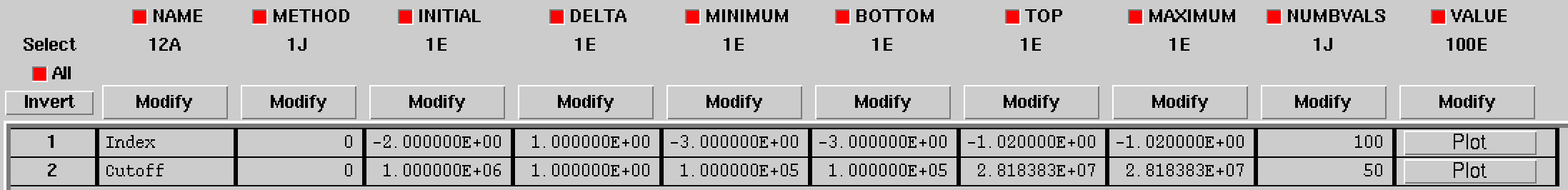
The PARAMETERS extension contains the definition of the model parameters.
Each row defines one model parameter. Each model parameter is defined by a
unique NAME. The METHOD column indicates whether the model should be
interpolated linarly (value 0) or logarithmically (value 1).
So far only linear interpolation is supported, hence the field is ignored.
The INITIAL column indicates the initial parameter value, if the value in
the DELTA column is negative the parameter will be fixed, otherwise it will
be fitted. The MINIMUM and MAXIMUM columns indicate the range of values
for a given parameter, the BOTTOM and TOP columns are ignored.
The``NUMBVALS`` column indicates the number of parameter values for
which the table model was computed, the VALUE column indicates the
specific parameter values.
In the example below there are two parameters named Index and Cutoff,
and spectra were computed for 100 index values and 50 cutoff values, hence
a total of 5000 spectra are stored in the table model.
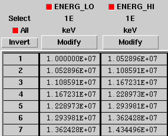
The SPECTRA extension contains the spectra of the table model. It consists
of two vector columns. The PARAMVAL column provides the parameter values
for which the spectrum was computed. Since there are two parameters in the
example the vector column has two entries. The INTPSPEC column provides
the spectrum \(\frac{dN(p)}{dE}\) for the specific parameters. Since there
are 200 energy bins in this example the vector column has 200 entries.
If the file name is given without a path it is expected that the file
resides in the same directory than the XML file.
If the file resides in a different directory, an absolute path name should
be specified.
Any environment variable present in the path name will be expanded.
Note that the default parameters of the table model are provided in the FITS
file, according to the
HEASARC OGIP standard.
However, table model parameters may also be specified in the XML file, and
these parameters will then overwrite the parameters in the FITS file. For
example, for a 2-dimensional table model with an Index and a Cutoff
parameter, the XML file may look like
where \(M_{\rm spectral}^{(i)}(E)\) is any spectral model component
(including another composite model), and \(N\) is the number of
model components that are combined.
where \(M_{\rm spectral}^{(i)}(E)\) is any spectral model component
(including another composite model), and \(N\) is the number of
model components that are multiplied.
\(M_{\rm spectral}(E)\) is any spectral model component
\(\alpha\) = Normalization
The model can be used to describe a spectrum with EBL absorption based on a
tabulated model of opacity as a function of photon energy. The corresponding
XML file structure for such a model is shown below:
the first block/factor corresponds to a power law;
the second block/factor models EBL absorption, and it points to an
ASCII file with two columns containing energy in \({\rm MeV}\)
as first column and opacity \(\tau\) as second column, respectively;
the parameter \(\alpha\) = Normalization represents an
opacity scaling factor.
Note
The Exponential model implements the function \(y=\exp(x)\),
hence in the example the scale attribute of the Normalization
parameter was set to -1 to implement the form
\(y=\exp(-x)\).