How to determine the extension of a source?

What you will learn

You will learn how you determine the spatial extent of a source by fitting an extended source model to the data.

To determine the spatial extension of a source, an extended source model has to be used in the model definition file for the source of interest. The example below is based on the source model that was determined during the iterative model improvement of the first CTA Data Challenge tutorial where two point sources were detected. As in the tutorial, Src001 is modelled with an exponentially cut-off power law spectrum, Src002 with a simple power law. In addition, a diffuse emission component was added to the model.

As noted during the iterative improvement of the source model there is a bright extended source south-west of the Galactic Centre, and we add now an additional Src003 component with a RadialDisk model to describe the spatial morphology of the source. To do this, copy the 1DC model definition file

$ cp $CTOOLS/share/models/1dc_howto.xml extended_model.xml

to extended_model.xml and add the following source to it:

  <source name="Src003" type="ExtendedSource" tscalc="1">
    <spectrum type="PowerLaw">
      <parameter name="Prefactor"   scale="5.7e-18" value="1.0" min="0"    max="1000.0" free="1"/>
      <parameter name="Index"       scale="-2.48"   value="1.0" min="-4.0" max="4.0"    free="1"/>
      <parameter name="PivotEnergy" scale="300000"  value="1.0" free="0" />
    </spectrum>
    <spatialModel type="RadialDisk">
      <parameter name="RA"     scale="1.0" value="266.3070" min="-360"  max="360" free="1"/>
      <parameter name="DEC"    scale="1.0" value="-30.1876" min="-90"   max="90"  free="1"/>
      <parameter name="Radius" scale="1.0" value="0.3"      min="0.001" max="10"  free="1"/>
    </spatialModel>
  </source>

Then run ctlike to fit the parameters of Src003 together with the other source parameters

$ ctlike
Input event list, counts cube or observation definition XML file [events.fits] cntcube.fits
Input exposure cube file [NONE] expcube.fits
Input PSF cube file [NONE] psfcube.fits
Input background cube file [NONE] bkgcube.fits
Input model definition XML file [$CTOOLS/share/models/crab.xml] extended_model.xml
Output model definition XML file [crab_results.xml] result.xml

The results can be seen in the log file and will also be written into the output model definition file. For illustration, an excerpt of the ctlike log file is shown below. The disk with of Src003 has been fitted to 0.326 +/- 0.005 degrees. The source is detected with a TS value of 960.3.

2019-04-04T10:02:58: === GModelSky ===
2019-04-04T10:02:58:  Name ......................: Src003
2019-04-04T10:02:58:  Instruments ...............: all
2019-04-04T10:02:58:  Test Statistic ............: 960.322220887407
2019-04-04T10:02:58:  Observation identifiers ...: all
2019-04-04T10:02:58:  Model type ................: ExtendedSource
2019-04-04T10:02:58:  Model components ..........: "RadialDisk" * "PowerLaw" * "Constant"
2019-04-04T10:02:58:  Number of parameters ......: 7
2019-04-04T10:02:58:  Number of spatial par's ...: 3
2019-04-04T10:02:58:   RA .......................: 266.317422676847 +/- 0.00715320609048925 [-360,360] deg (free,scale=1)
2019-04-04T10:02:58:   DEC ......................: -30.1850853839605 +/- 0.00616458713967605 [-90,90] deg (free,scale=1)
2019-04-04T10:02:58:   Radius ...................: 0.325736814893164 +/- 0.00480422517891009 [0.001,10] deg (free,scale=1)
2019-04-04T10:02:58:  Number of spectral par's ..: 3
2019-04-04T10:02:58:   Prefactor ................: 5.63906592494167e-17 +/- 6.89890876156083e-18 [0,5.7e-15] ph/cm2/s/MeV (free,scale=5.7e-18,gradient)
2019-04-04T10:02:58:   Index ....................: -2.7048301145616 +/- 0.0560202225832113 [9.92,-9.92]  (free,scale=-2.48,gradient)
2019-04-04T10:02:58:   PivotEnergy ..............: 300000 MeV (fixed,scale=300000,gradient)
2019-04-04T10:02:58:  Number of temporal par's ..: 1
2019-04-04T10:02:58:   Normalization ............: 1 (relative value) (fixed,scale=1,gradient)
2019-04-04T10:02:58:  Number of scale par's .....: 0

Warning

The parameter errors returned by ctlike are purely statistical. In addition to the statistical errors there are systematic uncertainties, such as for example the limits on the knowledge of the point spread function. These systematic uncertainties are not determined by ctools.

Now generate a residual map using csresmap to check the fit quality

$ csresmap
Input event list, counts cube, or observation definition XML file [events.fits] cntcube.fits
Input model cube file (generated with ctmodel) [NONE]
Input exposure cube file [NONE] expcube.fits
Input PSF cube file [NONE] psfcube.fits
Input background cube file [NONE] bkgcube.fits
Input model definition XML file [$CTOOLS/share/models/crab.xml] result.xml
Residual map computation algorithm (SUB|SUBDIV|SUBDIVSQRT|SIGNIFICANCE) [SIGNIFICANCE]
Output residual map file [resmap.fits]

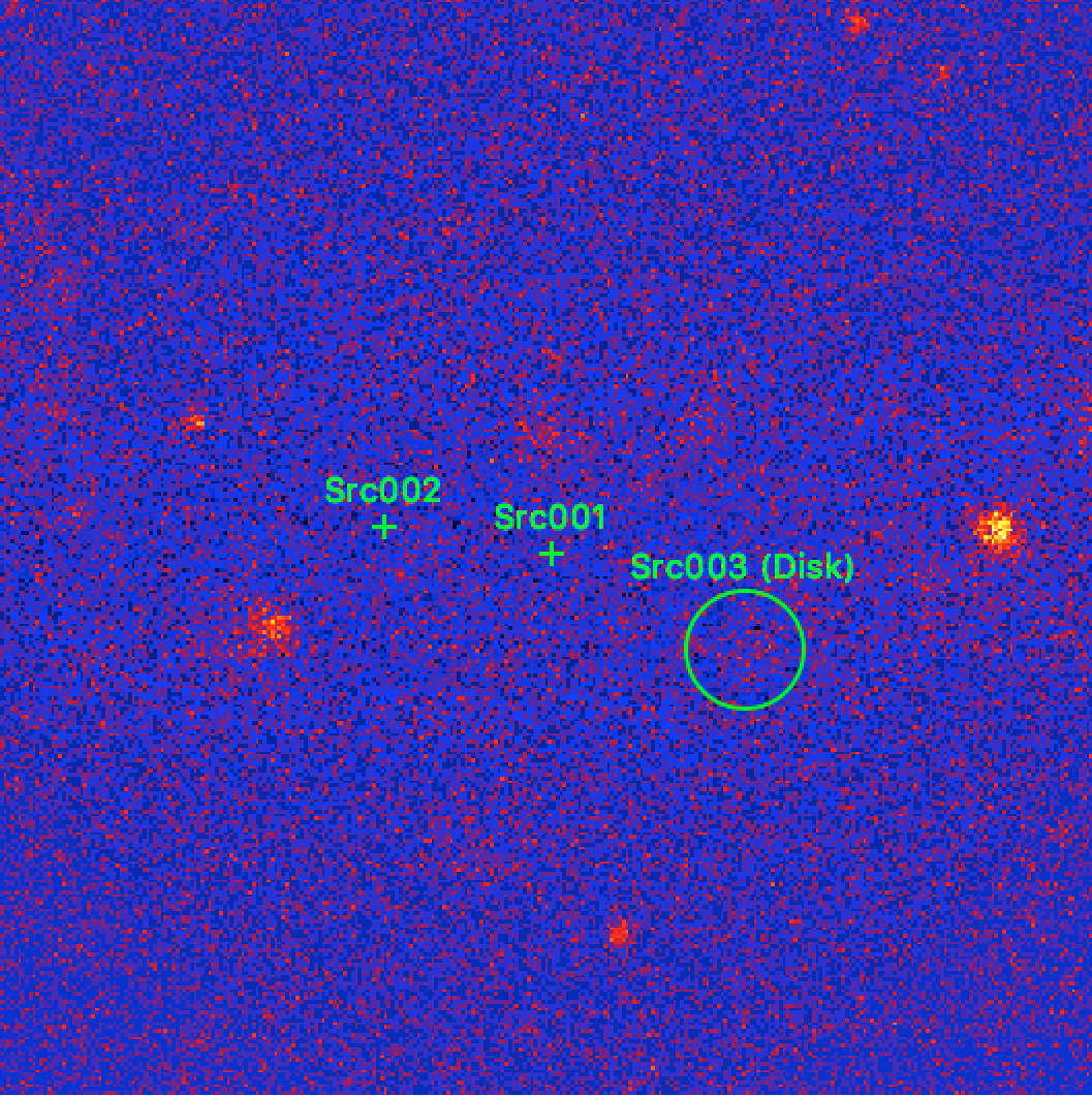
The resulting residual map is shown below. The map looks rather clean.

Residual sky map for a radial disk spatial shape for Src003

Tip

The region overlays for the residual sky maps were generated using the csmodelinfo script

$ csmodelinfo
Input model definition XML file [model.xml] result.xml
Output DS9 region file [ds9.reg] result.reg

Warning

The fitting of extended spatial models takes more computing time than the fitting of point sources. The computing time is related to the spatial extent of the source and to the spatial shape, with a Gaussian disk model taking considerably more computing time than a radial disk model due to the tails of the Gaussian function. It is therefore recommended to use by default radial disk models for the extension fitting, and only switch to a Gaussian disk models when really needed, or for the determination of final values for a publication.